

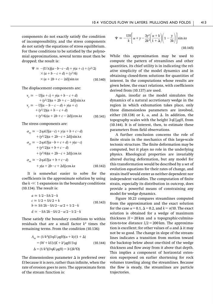
components do not exactly satisfy the condition
of incompressibility, and the stress components
do not satisfy the equations of stress equilibrium.
For these conditions to be satisfied by the polynomial approximations, several terms must then be
dropped; the result is:
(10.140)
The displacement components are:
(10.141)
The stress components are:
(10.142)
It is somewhat easier to solve for the
coefficients in the approximate solution by using
the k Ͻ Ͻ 1 expansions in the boundary conditions
(10.134). The result is:
(10.143)
These satisfy the boundary conditions to within
residuals that are a small factor k
2 times the
remaining terms. From the condition (10.136):
(10.144)
The dimensionless parameter ⌬ is preferred over
⍀ because it is zero, rather than infinite, when the
rate of erosion goes to zero. The approximate form
of the stream function is:
⌬ ϭ (1րk 2 )(3KրgH) ϭ 3ր(2k 2 ⍀)
ϭ (W ϩ kU)ր(K ϩ k 2 gHր3)
A ss Х (1րk 2 )(3UրgH)(␣ ϩ k)ր(1 ϩ ⌬)
d Х ϪSAր2kϪSAր2Ϫ␣ր2Ϫ1ր2Ϫk
b Х SAր2kϪSAր2Ϫ␣ր2 ϩ 1ր2Ϫk
c Х 1ր2 ϩ SAր2 ϩ k
a Х 1ր2ϪSAր2Ϫk
ϩ y(a ϩ 2bϪc ϩ 2d)] cos x
xx Х Ϫ2U[(a ϩ b ϩ cϪd)
ϩ (y 3 ր6)(a ϩ 2bϪc ϩ 2d)] cos x
ϩ (y 2 ր2)(a ϩ b ϩ c Ϫ d)
yy Х Ϫ2U[(aϪb ϩ c ϩ d) ϩ y(aϪc)
ϩ (y 2 ր2)(a ϩ 2bϪc ϩ 2d)] sin x
xy Х Ϫ2U[(aϪc) ϩ y (a ϩ b ϩ cϪd)
ϩ (y 3 ր6) (a ϩ 2b ϩ c Ϫ 2d)] cos x
ϩ (y 2 ր2)(a ϩ b Ϫ c ϩ d)
v y Х Ϫ U[(a Ϫ b Ϫ c Ϫ d) ϩ y(a ϩ c)
ϩ (y 2 ր2)(a ϩ 2b ϩ c Ϫ 2d)] sin x
v x Х Ϫ U[(a ϩ c) ϩ y(a ϩ b Ϫ c ϩ d)
ϫ (a ϩ 2b ϩ c Ϫ 2d)] sin x
ϫ (a ϩ b Ϫ c ϩ d) ϩ ( y 3 ր6)
⌿ Х Ϫ(Uր)[(aϪbϪcϪd) ϩ y(a ϩ c) ϩ ( y 2 ր2)
(10.145)
While this approximation may be used to
compute the pattern of streamlines and other
quantities, its chief utility is in indicating the relative simplicity of the model dynamics and in
obtaining closed-form solutions for quantities of
interest. In the computations whose results are
given below, the exact relations, with coefficients
derived from (10.137) are used.
Again, insofar as the model simulates the
dynamics of a natural accretionary wedge in the
region in which exhumation takes place, only
three dimensionless parameters are involved,
either (10.138) or k, ␣, and ⌬. In addition, the
topography scales with the height 3U/gH, from
(10.144). It is of interest, then, to estimate these
parameters from field observations.
A further conclusion concerns the role of
finite strain in the mechanics of this large-scale
tectonic structure. The finite deformation may be
computed, but it plays no role in the underlying
physics. Rheological properties are invariably
altered during deformation, but any model for
this transformation would be described by a set of
evolution equations for their rates of change, and
strain itself would enter as neither dependent nor
independent variables. The computation of finite
strain, especially its distribution in outcrop, does
provide a powerful means of constraining any
model for wedge dynamics.
Figure 10.23 compares streamlines computed
from the approximation and the exact solution
for the case ␣ ϭ 0.1, ⌬ϭ0.2, and k ϭ /10. The exact
solution is obtained for a wedge of maximum
thickness H ϭ 20 km and a topographic-culmination-to-toe distance L/2 ϭ 200 km. The approximation is excellent; for other values of ␣ and ⌬ it may
not be so good. The change in slope of the streamlines indicates a transition from motion toward
the backstop below about one-third of the wedge
thickness and flow away from it above that depth.
This implies a component of horizontal extension superposed on earlier shortening for rock
volumes traveling along the streamlines. Because
the flow is steady, the streamlines are particle
trajectories.
⌿ Х Ϫ
UH
k ΄ ␣ ϩ y Ϫ
3y 2
2k 2
␣ ϩ k
1 ϩ ⌬ 1 Ϫ
y
3k ΅ sin x
10.4 VISCOUS FLOW IN LAYERS: MULLIONS AND FOLDS
413
of incompressibility, and the stress components
do not satisfy the equations of stress equilibrium.
For these conditions to be satisfied by the polynomial approximations, several terms must then be
dropped; the result is:
(10.140)
The displacement components are:
(10.141)
The stress components are:
(10.142)
It is somewhat easier to solve for the
coefficients in the approximate solution by using
the k Ͻ Ͻ 1 expansions in the boundary conditions
(10.134). The result is:
(10.143)
These satisfy the boundary conditions to within
residuals that are a small factor k
2 times the
remaining terms. From the condition (10.136):
(10.144)
The dimensionless parameter ⌬ is preferred over
⍀ because it is zero, rather than infinite, when the
rate of erosion goes to zero. The approximate form
of the stream function is:
⌬ ϭ (1րk 2 )(3KրgH) ϭ 3ր(2k 2 ⍀)
ϭ (W ϩ kU)ր(K ϩ k 2 gHր3)
A ss Х (1րk 2 )(3UրgH)(␣ ϩ k)ր(1 ϩ ⌬)
d Х ϪSAր2kϪSAր2Ϫ␣ր2Ϫ1ր2Ϫk
b Х SAր2kϪSAր2Ϫ␣ր2 ϩ 1ր2Ϫk
c Х 1ր2 ϩ SAր2 ϩ k
a Х 1ր2ϪSAր2Ϫk
ϩ y(a ϩ 2bϪc ϩ 2d)] cos x
xx Х Ϫ2U[(a ϩ b ϩ cϪd)
ϩ (y 3 ր6)(a ϩ 2bϪc ϩ 2d)] cos x
ϩ (y 2 ր2)(a ϩ b ϩ c Ϫ d)
yy Х Ϫ2U[(aϪb ϩ c ϩ d) ϩ y(aϪc)
ϩ (y 2 ր2)(a ϩ 2bϪc ϩ 2d)] sin x
xy Х Ϫ2U[(aϪc) ϩ y (a ϩ b ϩ cϪd)
ϩ (y 3 ր6) (a ϩ 2b ϩ c Ϫ 2d)] cos x
ϩ (y 2 ր2)(a ϩ b Ϫ c ϩ d)
v y Х Ϫ U[(a Ϫ b Ϫ c Ϫ d) ϩ y(a ϩ c)
ϩ (y 2 ր2)(a ϩ 2b ϩ c Ϫ 2d)] sin x
v x Х Ϫ U[(a ϩ c) ϩ y(a ϩ b Ϫ c ϩ d)
ϫ (a ϩ 2b ϩ c Ϫ 2d)] sin x
ϫ (a ϩ b Ϫ c ϩ d) ϩ ( y 3 ր6)
⌿ Х Ϫ(Uր)[(aϪbϪcϪd) ϩ y(a ϩ c) ϩ ( y 2 ր2)
(10.145)
While this approximation may be used to
compute the pattern of streamlines and other
quantities, its chief utility is in indicating the relative simplicity of the model dynamics and in
obtaining closed-form solutions for quantities of
interest. In the computations whose results are
given below, the exact relations, with coefficients
derived from (10.137) are used.
Again, insofar as the model simulates the
dynamics of a natural accretionary wedge in the
region in which exhumation takes place, only
three dimensionless parameters are involved,
either (10.138) or k, ␣, and ⌬. In addition, the
topography scales with the height 3U/gH, from
(10.144). It is of interest, then, to estimate these
parameters from field observations.
A further conclusion concerns the role of
finite strain in the mechanics of this large-scale
tectonic structure. The finite deformation may be
computed, but it plays no role in the underlying
physics. Rheological properties are invariably
altered during deformation, but any model for
this transformation would be described by a set of
evolution equations for their rates of change, and
strain itself would enter as neither dependent nor
independent variables. The computation of finite
strain, especially its distribution in outcrop, does
provide a powerful means of constraining any
model for wedge dynamics.
Figure 10.23 compares streamlines computed
from the approximation and the exact solution
for the case ␣ ϭ 0.1, ⌬ϭ0.2, and k ϭ /10. The exact
solution is obtained for a wedge of maximum
thickness H ϭ 20 km and a topographic-culmination-to-toe distance L/2 ϭ 200 km. The approximation is excellent; for other values of ␣ and ⌬ it may
not be so good. The change in slope of the streamlines indicates a transition from motion toward
the backstop below about one-third of the wedge
thickness and flow away from it above that depth.
This implies a component of horizontal extension superposed on earlier shortening for rock
volumes traveling along the streamlines. Because
the flow is steady, the streamlines are particle
trajectories.
⌿ Х Ϫ
UH
k ΄ ␣ ϩ y Ϫ
3y 2
2k 2
␣ ϩ k
1 ϩ ⌬ 1 Ϫ
y
3k ΅ sin x
10.4 VISCOUS FLOW IN LAYERS: MULLIONS AND FOLDS
413