

take place on both sides of this. A very simple
modification of the present model may be made
to account for this, but we avoid the temptation to
introduce it in order to achieve the simplest
approximation to wedge dynamics. Moreover, the
effect of any such modification to a model is best
appreciated by first studying the behavior before
it is introduced.
Prior to solving (10.134), we consider the
special restriction to the case of a steady-state
wedge, in which the amount of material lost by
erosion and outward flow is just balanced by the
inward flow, and the balance is achieved by timeindependent regimens of influx, underplating,
and erosion. For the present model, this requires
that the vertical flux of material in the interval of
interest, 0 Յ x Յ L/4, and at the upper surface, is
just balanced by erosion. We use a rate of erosion
proportional to the local topographic relief
which, in view of the sinusoidal variation of
topography, is described by:
(10.135)
In the steady state, this loss is just balanced by the
flux associated with v y (x, H) over the same interval
in x. This gives the condition:
(10.136)
Here A ss is the amplitude of the steady-state topographic relief.
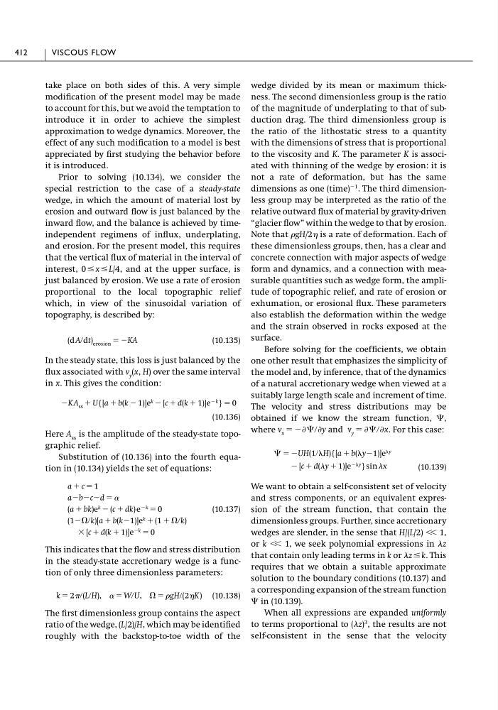
Substitution of (10.136) into the fourth equation in (10.134) yields the set of equations:
(10.137)
This indicates that the flow and stress distribution
in the steady-state accretionary wedge is a function of only three dimensionless parameters:
(10.138)
The first dimensionless group contains the aspect
ratio of the wedge, (L/2)/H, which may be identified
roughly with the backstop-to-toe width of the
k ϭ 2ր(LրH), ␣ ϭ WրU, ⍀ ϭ gHր(2K )
ϫ [c ϩ d(k ϩ 1)]e Ϫk ϭ 0
(1Ϫ⍀րk)[a ϩ b(kϪ1)]e k ϩ (1 ϩ ⍀րk)
(a ϩ bk)e k Ϫ (c ϩ dk) e Ϫk ϭ 0
aϪbϪcϪd ϭ ␣
a ϩ c ϭ 1
ϪK A ss ϩ U{[a ϩ b(k Ϫ 1)]e k Ϫ [c ϩ d(k ϩ 1)]e Ϫk } ϭ 0
(d Aրdt) erosion ϭ ϪKA
wedge divided by its mean or maximum thickness. The second dimensionless group is the ratio
of the magnitude of underplating to that of subduction drag. The third dimensionless group is
the ratio of the lithostatic stress to a quantity
with the dimensions of stress that is proportional
to the viscosity and K. The parameter K is associated with thinning of the wedge by erosion: it is
not a rate of deformation, but has the same
dimensions as one (time)
Ϫ1 . The third dimensionless group may be interpreted as the ratio of the
relative outward flux of material by gravity-driven
“glacier flow” within the wedge to that by erosion.
Note that gH/2 is a rate of deformation. Each of
these dimensionless groups, then, has a clear and
concrete connection with major aspects of wedge
form and dynamics, and a connection with measurable quantities such as wedge form, the amplitude of topographic relief, and rate of erosion or
exhumation, or erosional flux. These parameters
also establish the deformation within the wedge
and the strain observed in rocks exposed at the
surface.
Before solving for the coefficients, we obtain
one other result that emphasizes the simplicity of
the model and, by inference, that of the dynamics
of a natural accretionary wedge when viewed at a
suitably large length scale and increment of time.
The velocity and stress distributions may be
obtained if we know the stream function, ⌿,
where
For this case:
(10.139)
We want to obtain a self-consistent set of velocity
and stress components, or an equivalent expression of the stream function, that contain the
dimensionless groups. Further, since accretionary
wedges are slender, in the sense that H/(L/2) Ͻ Ͻ 1,
or k Ͻ Ͻ 1, we seek polynomial expressions in z
that contain only leading terms in k or z Յ k. This
requires that we obtain a suitable approximate
solution to the boundary conditions (10.137) and
a corresponding expansion of the stream function
⌿ in (10.139).
When all expressions are expanded uniformly
to terms proportional to (z)
3 , the results are not
self-consistent in the sense that the velocity
Ϫ [c ϩ d(y ϩ 1)]e Ϫy } sin x
⌿ ϭ ϪUH(1րH){[a ϩ b(yϪ1)]e y
v x ϭ ϪѨ⌿րѨy and v y ϭ Ѩ⌿րѨx.
412
VISCOUS FLOW
modification of the present model may be made
to account for this, but we avoid the temptation to
introduce it in order to achieve the simplest
approximation to wedge dynamics. Moreover, the
effect of any such modification to a model is best
appreciated by first studying the behavior before
it is introduced.
Prior to solving (10.134), we consider the
special restriction to the case of a steady-state
wedge, in which the amount of material lost by
erosion and outward flow is just balanced by the
inward flow, and the balance is achieved by timeindependent regimens of influx, underplating,
and erosion. For the present model, this requires
that the vertical flux of material in the interval of
interest, 0 Յ x Յ L/4, and at the upper surface, is
just balanced by erosion. We use a rate of erosion
proportional to the local topographic relief
which, in view of the sinusoidal variation of
topography, is described by:
(10.135)
In the steady state, this loss is just balanced by the
flux associated with v y (x, H) over the same interval
in x. This gives the condition:
(10.136)
Here A ss is the amplitude of the steady-state topographic relief.
Substitution of (10.136) into the fourth equation in (10.134) yields the set of equations:
(10.137)
This indicates that the flow and stress distribution
in the steady-state accretionary wedge is a function of only three dimensionless parameters:
(10.138)
The first dimensionless group contains the aspect
ratio of the wedge, (L/2)/H, which may be identified
roughly with the backstop-to-toe width of the
k ϭ 2ր(LրH), ␣ ϭ WրU, ⍀ ϭ gHր(2K )
ϫ [c ϩ d(k ϩ 1)]e Ϫk ϭ 0
(1Ϫ⍀րk)[a ϩ b(kϪ1)]e k ϩ (1 ϩ ⍀րk)
(a ϩ bk)e k Ϫ (c ϩ dk) e Ϫk ϭ 0
aϪbϪcϪd ϭ ␣
a ϩ c ϭ 1
ϪK A ss ϩ U{[a ϩ b(k Ϫ 1)]e k Ϫ [c ϩ d(k ϩ 1)]e Ϫk } ϭ 0
(d Aրdt) erosion ϭ ϪKA
wedge divided by its mean or maximum thickness. The second dimensionless group is the ratio
of the magnitude of underplating to that of subduction drag. The third dimensionless group is
the ratio of the lithostatic stress to a quantity
with the dimensions of stress that is proportional
to the viscosity and K. The parameter K is associated with thinning of the wedge by erosion: it is
not a rate of deformation, but has the same
dimensions as one (time)
Ϫ1 . The third dimensionless group may be interpreted as the ratio of the
relative outward flux of material by gravity-driven
“glacier flow” within the wedge to that by erosion.
Note that gH/2 is a rate of deformation. Each of
these dimensionless groups, then, has a clear and
concrete connection with major aspects of wedge
form and dynamics, and a connection with measurable quantities such as wedge form, the amplitude of topographic relief, and rate of erosion or
exhumation, or erosional flux. These parameters
also establish the deformation within the wedge
and the strain observed in rocks exposed at the
surface.
Before solving for the coefficients, we obtain
one other result that emphasizes the simplicity of
the model and, by inference, that of the dynamics
of a natural accretionary wedge when viewed at a
suitably large length scale and increment of time.
The velocity and stress distributions may be
obtained if we know the stream function, ⌿,
where
For this case:
(10.139)
We want to obtain a self-consistent set of velocity
and stress components, or an equivalent expression of the stream function, that contain the
dimensionless groups. Further, since accretionary
wedges are slender, in the sense that H/(L/2) Ͻ Ͻ 1,
or k Ͻ Ͻ 1, we seek polynomial expressions in z
that contain only leading terms in k or z Յ k. This
requires that we obtain a suitable approximate
solution to the boundary conditions (10.137) and
a corresponding expansion of the stream function
⌿ in (10.139).
When all expressions are expanded uniformly
to terms proportional to (z)
3 , the results are not
self-consistent in the sense that the velocity
Ϫ [c ϩ d(y ϩ 1)]e Ϫy } sin x
⌿ ϭ ϪUH(1րH){[a ϩ b(yϪ1)]e y
v x ϭ ϪѨ⌿րѨy and v y ϭ Ѩ⌿րѨx.
412
VISCOUS FLOW