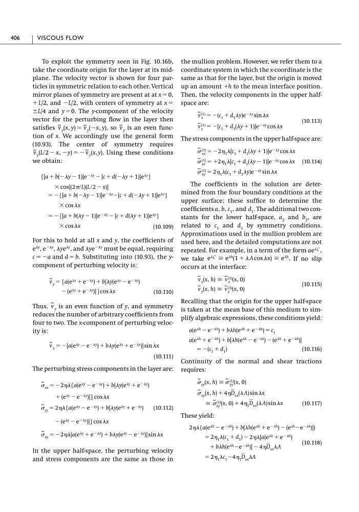
To exploit the symmetry seen in Fig. 10.16b,
take the coordinate origin for the layer at its midplane. The velocity vector is shown for four particles in symmetric relation to each other. Vertical
mirror planes of symmetry are present at at x ϭ 0,
ϩL/2, and ϪL/2, with centers of symmetry at x ϭ
ϮL/4 and y ϭ 0. The y-component of the velocity
vector for the perturbing flow in the layer then
satisfies
, so
is an even function of x. We accordingly use the general form
(10.93). The center of symmetry requires
Using these conditions
we obtain:
(10.109)
For this to hold at all x and y, the coefficients of
e ␭y , e Ϫ␭y , ␭ye ␭y , and ␭ye
Ϫ␭y must be equal, requiring
. Substituting into (10.93), the ycomponent of perturbing velocity is:
(10.110)
Thus,
is an even function of y, and symmetry
reduces the number of arbitrary coefficients from
four to two. The x-component of perturbing velocity is:
(10.111)
The perturbing stress components in the layer are:
(10.112)
In the upper half-space, the perturbing velocity
and stress components are the same as those in
␴
~ xy ϭ Ϫ2␩␭[a(e ␭y ϩ e Ϫ␭y ) ϩ b␭y(e ␭y Ϫ e Ϫ␭y )] sin ␭x
Ϫ (e ␭y Ϫ e Ϫ␭y )]} cos ␭x
␴
~ yy ϭ 2␩␭{a(e ␭y Ϫ e Ϫ␭y ) ϩ b[␭y(e ␭y ϩ e Ϫ␭y )
ϩ (e ␭y Ϫ e Ϫ␭y )]} cos ␭x
␴
~ xx ϭ Ϫ2␩␭{a(e ␭y Ϫ e Ϫ␭y ) ϩ b[␭y(e ␭y ϩ e Ϫ␭y )
v
~ x ϭ Ϫ[a(e ␭y Ϫ e Ϫ␭y ) ϩ b␭y(e ␭y ϩ e Ϫ␭y )] sin ␭x
v
~ y
Ϫ (e ␭y ϩ e Ϫ␭y )] }cos ␭x
v
~ y ϭ {a(e ␭y ϩ e Ϫ␭y ) ϩ b[␭y(e ␭y Ϫ e Ϫ␭y )
c ϭ Ϫa and d ϭ b
ϫ cos ␭x
ϭ Ϫ{[a ϩ b(␭y Ϫ 1)]e Ϫ␭y Ϫ [c ϩ d(␭y ϩ 1)]e ␭y }
ϫ cos ␭x
ϭ Ϫ{[a ϩ b(Ϫ␭y Ϫ 1)]e Ϫ␭y Ϫ[c ϩ d(Ϫ␭y ϩ 1)]e ␭y }
ϫ cos[(2␲րL)(L ր2 Ϫ x)]
{[a ϩ b(Ϫ␭y Ϫ 1)]e Ϫ␭y Ϫ [c ϩ d(Ϫ␭y ϩ 1)]e ␭y }
v
~ y (Lր2 Ϫ x, Ϫy) ϭ Ϫ v
~ y (x, y).
v
~ y
v
~ y (x, y) ϭ v
~ y (Ϫx, y)
the mullion problem. However, we refer them to a
coordinate system in which the x-coordinate is the
same as that for the layer, but the origin is moved
up an amount ϩh to the mean interface position.
Then, the velocity components in the upper halfspace are:
(10.113)
The stress components in the upper half-space are:
(10.114)
The coefficients in the solution are determined from the four boundary conditions at the
upper surface; these suffice to determine the
coefficients
The additional two constants for the lower half-space, a 2 and b 2 , are
related to c 1 and d 1 by symmetry conditions.
Approximations used in the mullion problem are
used here, and the detailed computations are not
repeated. For example, in a term of the form
we take
If no slip
occurs at the interface:
(10.115)
Recalling that the origin for the upper half-space
is taken at the mean base of this medium to simplify algebraic expressions, these conditions yield:
(10.116)
Continuity of the normal and shear tractions
requires:
(10.117)
These yield:
(10.118)
ϭ 2␩ 1 ␭c 1 Ϫ4␩ 1 D xx ␭A
Ϫ 4␩D xx ␭A
ϩ b␭h(e ␭h Ϫe Ϫ␭h )]
Ϫ 2␩␭[a(e ␭h ϩ e Ϫ␭h )
ϭ 2␩ 1 ␭(c 1 ϩ d 1 )
Ϫ (e ␭h Ϫe Ϫ␭h )])
2␩␭{a(e ␭h Ϫ e Ϫ␭h ) ϩ b[␭h(e ␭h ϩ e Ϫ␭h )
ϩ 4␩ 1 D xx (␭ A) sin ␭x
Х ␴
~ (1)
xy (x, 0)
␴
~ xy (x, h) ϩ 4␩D xx (␭ A) sin ␭x
␴
~ yy (x, h) Х ␴
~ (1)
yy (x, 0)
ϭ Ϫ(c 1 ϩ d 1 )
a(e ␭h ϩ e Ϫ␭h ) ϩ b[␭h(e ␭h Ϫ e Ϫ␭h ) Ϫ (e ␭h ϩ e Ϫ␭h )]
a(e ␭h Ϫ e Ϫ␭h ) ϩ b␭h(e ␭h ϩ e Ϫ␭h ) ϭ c 1
v
~ y (x, h) Х v
~ (1)
y (x, 0)
v
~ x (x, h) Х v
~ (1)
x (x, 0)
e ␭␨Ј Х e ␭h (1 ϩ ␭ A cos ␭x) Х e ␭h .
ae ␭␨Ј ,
a, b, c 1 , and d 1 .
␴
~ (1)
xy ϭ 2␩ 1 ␭(c 1 ϩ d 1 ␭y)e Ϫ␭y sin ␭x
␴
~ (1)
yy ϭ ϩ2␩ 1 ␭[c 1 ϩ d 1 (␭y Ϫ 1)]e Ϫ␭y cos ␭x
␴
~ (1)
xx ϭ Ϫ2␩ 1 ␭[c 1 ϩ d 1 (␭y ϩ 1)]e Ϫ␭y cos ␭x
v
~ (1)
y ϭ Ϫ[c 1 ϩ d 1 (␭y ϩ 1)]e Ϫ␭y cos ␭x
v
~ (1)
x ϭ Ϫ(c 1 ϩ d 1 ␭y)e Ϫ␭y sin ␭x
406
VISCOUS FLOW