

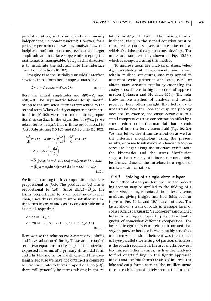
present solution, such components are linearly
independent, i.e. non-interacting. However, for a
periodic perturbation, we may analyze how the
incipient mullion structure evolves at larger
amplitude and interface slope while keeping the
mathematics manageable. A step in this direction
is to substitute the solution into the interface
evolution equation (10.102).
Imagine that the initially sinusoidal interface
develops into a form better approximated by:
(10.103)
Here the initial amplitudes are A(0) ϭ A 0 and
AЈ(0) ϭ 0. The asymmetric lobe-and-cusp modification to the sinusoidal form is represented by the
second term. When velocity components are substituted in (10.102), we retain contributions proportional to cos 2x. In the expansion of
we
retain terms in a 2 , that is those proportional to
(A)
2 . Substituting (10.103) and (10.98) into (10.102):
(1.104)
We find, according to this computation, that AЈ is
proportional to (A)
2 . The product a 2 (A) also is
proportional to (A)
2 . Since
the
terms proportional to x on both sides cancel.
Then, since this relation must be satisfied at all x,
the terms in cos x and cos 2x on each side must
be equal, requiring:
(10.105)
Here we use the relation cos 2x ϭ cos
2 x Ϫ sin
2 x
and have substituted for a 2 . These are a coupled
set of two equations in the shape of the interface
expressed in terms of a primary sinusoidal form
and a first-harmonic form with one-half the wavelength. Because we have not obtained a complete
solution accurate to terms proportional to (A)
2 ,
there will generally be terms missing in the redAЈրdt Х ϪD xx AЈϪ 2[(1 Ϫ R) ր(1 ϩ R)]D xx A( A)
dAրdt Х ϪD xx A
d րdt ϭ D xx ,
Ϫ (D xx x Ϫ a 2 sin x)(ϪA sin xϪ2 AЈsin 2x)
ϭ ϪD xx (A cos x ϩ AЈ cos 2x) ϩ a 2 (A cos x) cos x
ϪAЈ sin 2x 2x
d
dt
dA
dt
cos x Ϫ A sin x
x
d
dt
ϩ
dAЈ
dt
cos 2x
v (2)
y (x, ),
(x, t) ϭ A cos x ϩ AЈcos 2x
lation for dAЈ/dt. In fact, if the missing term is
included, the 2 in the second equation must be
cancelled so (10.105) over-estimates the rate at
which the lobe-and-cusp structure develops. The
more accurate result is shown in Fig. 10.13b,
which is computed using this method.
To improve upon the analysis of stress, velocity, morphological development, and strain
within mullion structures, one may appeal to
numerical codes (Dieterich and Onat, 1969), or
obtain more accurate results by extending the
analysis used here to higher orders of approximation (Johnson and Fletcher, 1994). The relatively simple method of analysis and results
provided here offers insight that helps us to
understand how the lobe-and-cusp morphology
develops. In essence, the cusps occur due to a
small compressive stress concentration offset by a
stress reduction in the material that extends
outward into the less viscous fluid (Fig. 10.12b).
We may follow the strain distribution as well as
the interface morphology using the present
results, or to see to what extent a tendency to preserve arc length along the interface exists. Both
the kinematics and the stress distribution
suggest that a variety of minor structures might
be formed close to the interface in a region of
marked strain variation.
10.4.3 Folding of a single viscous layer
The method of analysis developed in the preceding section may be applied to the folding of a
more viscous layer isolated in a less viscous
medium, giving insight into how folds such as
those in Fig. 10.1a and 10.14 are initiated. The
latter shows a train of folds in a single layer of
coarse K-feldspar/quartz “leucosome” sandwiched
between two layers of quartz–plagioclase–biotite
gneiss of somewhat different composition. The
layer is irregular, because either it formed that
way, in part, or because it was possibly stretched
in an irregular fashion before it was then folded
in layer-parallel shortening. Of particular interest
is the rough regularity in the arc lengths between
fold hinges. Other features, such as the tendency
to find quartz filling in the tightly appressed
hinges and the fold forms are also of interest. The
lobe-and-cusp forms seen in the mullion structures are also approximately seen in the forms of
10.4 VISCOUS FLOW IN LAYERS: MULLIONS AND FOLDS
403
independent, i.e. non-interacting. However, for a
periodic perturbation, we may analyze how the
incipient mullion structure evolves at larger
amplitude and interface slope while keeping the
mathematics manageable. A step in this direction
is to substitute the solution into the interface
evolution equation (10.102).
Imagine that the initially sinusoidal interface
develops into a form better approximated by:
(10.103)
Here the initial amplitudes are A(0) ϭ A 0 and
AЈ(0) ϭ 0. The asymmetric lobe-and-cusp modification to the sinusoidal form is represented by the
second term. When velocity components are substituted in (10.102), we retain contributions proportional to cos 2x. In the expansion of
we
retain terms in a 2 , that is those proportional to
(A)
2 . Substituting (10.103) and (10.98) into (10.102):
(1.104)
We find, according to this computation, that AЈ is
proportional to (A)
2 . The product a 2 (A) also is
proportional to (A)
2 . Since
the
terms proportional to x on both sides cancel.
Then, since this relation must be satisfied at all x,
the terms in cos x and cos 2x on each side must
be equal, requiring:
(10.105)
Here we use the relation cos 2x ϭ cos
2 x Ϫ sin
2 x
and have substituted for a 2 . These are a coupled
set of two equations in the shape of the interface
expressed in terms of a primary sinusoidal form
and a first-harmonic form with one-half the wavelength. Because we have not obtained a complete
solution accurate to terms proportional to (A)
2 ,
there will generally be terms missing in the redAЈրdt Х ϪD xx AЈϪ 2[(1 Ϫ R) ր(1 ϩ R)]D xx A( A)
dAրdt Х ϪD xx A
d րdt ϭ D xx ,
Ϫ (D xx x Ϫ a 2 sin x)(ϪA sin xϪ2 AЈsin 2x)
ϭ ϪD xx (A cos x ϩ AЈ cos 2x) ϩ a 2 (A cos x) cos x
ϪAЈ sin 2x 2x
d
dt
dA
dt
cos x Ϫ A sin x
x
d
dt
ϩ
dAЈ
dt
cos 2x
v (2)
y (x, ),
(x, t) ϭ A cos x ϩ AЈcos 2x
lation for dAЈ/dt. In fact, if the missing term is
included, the 2 in the second equation must be
cancelled so (10.105) over-estimates the rate at
which the lobe-and-cusp structure develops. The
more accurate result is shown in Fig. 10.13b,
which is computed using this method.
To improve upon the analysis of stress, velocity, morphological development, and strain
within mullion structures, one may appeal to
numerical codes (Dieterich and Onat, 1969), or
obtain more accurate results by extending the
analysis used here to higher orders of approximation (Johnson and Fletcher, 1994). The relatively simple method of analysis and results
provided here offers insight that helps us to
understand how the lobe-and-cusp morphology
develops. In essence, the cusps occur due to a
small compressive stress concentration offset by a
stress reduction in the material that extends
outward into the less viscous fluid (Fig. 10.12b).
We may follow the strain distribution as well as
the interface morphology using the present
results, or to see to what extent a tendency to preserve arc length along the interface exists. Both
the kinematics and the stress distribution
suggest that a variety of minor structures might
be formed close to the interface in a region of
marked strain variation.
10.4.3 Folding of a single viscous layer
The method of analysis developed in the preceding section may be applied to the folding of a
more viscous layer isolated in a less viscous
medium, giving insight into how folds such as
those in Fig. 10.1a and 10.14 are initiated. The
latter shows a train of folds in a single layer of
coarse K-feldspar/quartz “leucosome” sandwiched
between two layers of quartz–plagioclase–biotite
gneiss of somewhat different composition. The
layer is irregular, because either it formed that
way, in part, or because it was possibly stretched
in an irregular fashion before it was then folded
in layer-parallel shortening. Of particular interest
is the rough regularity in the arc lengths between
fold hinges. Other features, such as the tendency
to find quartz filling in the tightly appressed
hinges and the fold forms are also of interest. The
lobe-and-cusp forms seen in the mullion structures are also approximately seen in the forms of
10.4 VISCOUS FLOW IN LAYERS: MULLIONS AND FOLDS
403