

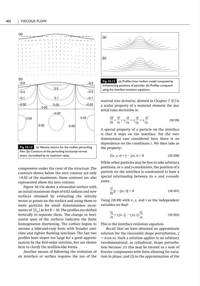
compressive under the crest of the structure. The
contours shown below the zero contour are only
Ϯ0.02 of the maximum; these contours are also
represented above the zero contour.
Figure 10.13a shows a sinusoidal surface with
an initial maximum slope of 0.02 radians and new
surfaces obtained by evaluating the velocity
vector at points on the surface and using them to
move particles for small dimensionless increments of
for R ϭ 10. The profiles are shifted
vertically to separate them. The change in horizontal span of the surfaces indicates the finite
homogeneous shortening. The surface begins to
assume a lobe-and-cusp form with broader anticline and tighter flanking synclines. The last two
profiles have slopes too large for a good approximation by the first-order solution, but are shown
here to clarify the mullion-like forms.
Another means of following the evolution of
an interface or surface requires the use of the
|D xx |⌬t
material time derivative, derived in Chapter 7. If f is
a scalar property of a material element the material time derivative is:
(10.99)
A special property of a particle on the interface
is that it stays on the interface. For the twodimensional case considered here there is no
dependence on the coordinate z. We then take as
the property:
(10.100)
While other particles may be free to take arbitrary
positions, or x- and y-coordinates, the position of a
particle on the interface is constrained to have a
special relationship between its x- and y-coordinates:
(10.101)
Using (10.99) with x, y, and t as the independent
variables we find:
(10.102)
This is the interface evolution equation.
Recall that we have obtained an approximate
solution for the sinusoidal shape perturbation,
ϭ Acos x. Such a solution applies to an arbitrary
two-dimensional, or cylindrical, shape perturbation because: (1) this may be treated as a sum of
Fourier components with form allowing for variation in phase; and (2) to the approximation of the
Ѩ
Ѩt
ϭ v y (x, ) Ϫ v x (x, )
Ѩ
Ѩx
D
Dt
[y Ϫ (x, t)] ϭ 0
f (x, y, t) ϭ y Ϫ (x, t) ϭ 0
Df
Dt
ϭ
Ѩf
Ѩt
ϩ v x
Ѩf
Ѩx
ϩ v y
Ѩf
Ѩy
ϩ v z
Ѩf
Ѩz
402
VISCOUS FLOW
Fig 10.12 (a) Velocity vectors for the mullion perturbing
flow. (b) Contours of the perturbing horizontal normal
stress, normalized by its maximum value.
(a)
(b)
–0.02
–0.02
0.00
0.02
0.02
0.02
0.00
0.00
–0.02
0.1
–0.1
–0.1
–0.5
0.5
–0.5
–0.9
–0.9
Fig 10.13 (a) Profiles from mullion model computed by
incrementing positions of particles. (b) Profiles computed
using the interface evolution equations.
(a)
(b)
contours shown below the zero contour are only
Ϯ0.02 of the maximum; these contours are also
represented above the zero contour.
Figure 10.13a shows a sinusoidal surface with
an initial maximum slope of 0.02 radians and new
surfaces obtained by evaluating the velocity
vector at points on the surface and using them to
move particles for small dimensionless increments of
for R ϭ 10. The profiles are shifted
vertically to separate them. The change in horizontal span of the surfaces indicates the finite
homogeneous shortening. The surface begins to
assume a lobe-and-cusp form with broader anticline and tighter flanking synclines. The last two
profiles have slopes too large for a good approximation by the first-order solution, but are shown
here to clarify the mullion-like forms.
Another means of following the evolution of
an interface or surface requires the use of the
|D xx |⌬t
material time derivative, derived in Chapter 7. If f is
a scalar property of a material element the material time derivative is:
(10.99)
A special property of a particle on the interface
is that it stays on the interface. For the twodimensional case considered here there is no
dependence on the coordinate z. We then take as
the property:
(10.100)
While other particles may be free to take arbitrary
positions, or x- and y-coordinates, the position of a
particle on the interface is constrained to have a
special relationship between its x- and y-coordinates:
(10.101)
Using (10.99) with x, y, and t as the independent
variables we find:
(10.102)
This is the interface evolution equation.
Recall that we have obtained an approximate
solution for the sinusoidal shape perturbation,
ϭ Acos x. Such a solution applies to an arbitrary
two-dimensional, or cylindrical, shape perturbation because: (1) this may be treated as a sum of
Fourier components with form allowing for variation in phase; and (2) to the approximation of the
Ѩ
Ѩt
ϭ v y (x, ) Ϫ v x (x, )
Ѩ
Ѩx
D
Dt
[y Ϫ (x, t)] ϭ 0
f (x, y, t) ϭ y Ϫ (x, t) ϭ 0
Df
Dt
ϭ
Ѩf
Ѩt
ϩ v x
Ѩf
Ѩx
ϩ v y
Ѩf
Ѩy
ϩ v z
Ѩf
Ѩz
402
VISCOUS FLOW
Fig 10.12 (a) Velocity vectors for the mullion perturbing
flow. (b) Contours of the perturbing horizontal normal
stress, normalized by its maximum value.
(a)
(b)
–0.02
–0.02
0.00
0.02
0.02
0.02
0.00
0.00
–0.02
0.1
–0.1
–0.1
–0.5
0.5
–0.5
–0.9
–0.9
Fig 10.13 (a) Profiles from mullion model computed by
incrementing positions of particles. (b) Profiles computed
using the interface evolution equations.
(a)
(b)