

Eliminating the two components of velocity
between them yields the rate of deformation compatibility relation:
(10.64)
In order to obtain this equation by taking partial
derivatives, and even before that to write the rate
of deformation components in terms of partial
derivatives of the velocity components, the velocity components must be continuous and have continuous partial derivatives to third order. This
continuity is a prior necessary condition for deriving (10.64). Structural geologists often refer to the
compatibility condition as a condition required to
insure that the velocity field (or displacement
field) is smooth, so that pieces of the body
described are not slipping or separating relative to
each other. This interpretation has things backwards: continuity is required to write down (10.64).
From (10.14) and (10.63) the rate of deformation components in terms of the stress function
are:
(10.65)
Substituting into (10.64), we find:
(10.66)
In the present case, we suppose that the viscosity,
, is not a function of position so we obtain:
(10.67)
This is the biharmonic equation, often written in the
condensed form:
(10.68)
Having reduced the general set of equations for
plane flow, (10.12)–(10.15), to a single equation in
one unknown function, (x, y), the next step is to
set up some boundary value problems of interest
and solve them.
ٌ 4 ϭ ٌ 2 (ٌ 2 ) ϭ 0
Ѩ 4
Ѩy 4 ϩ 2
Ѩ 4
Ѩy 2 Ѩx 2 ϩ
Ѩ 4
Ѩx 4 ϭ 0
Ϫ 2
Ѩ 2
ѨxѨy Ϫ
1
2
Ѩ 2
ѨxѨy ϭ 0
Ѩ 2
Ѩy 2 Ϫ
Ѩ 2
Ѩx 2 ΄
1
4
Ѩ 2
Ѩy 2 Ϫ
Ѩ 2
Ѩx 2 ΅
D xx ϭ ϪD yy ϭ
1
4
Ѩ 2
Ѩy 2 Ϫ
Ѩ 2
Ѩx 2
, D xy ϭ
1
2
Ѩ 2
ѨxѨy
Ѩ 2 D xx
Ѩy 2 Ϫ 2
Ѩ 2 Dxy
ѨxѨy
ϩ
Ѩ 2 Dyy
Ѩx 2 ϭ 0
10.4.2 Mullions
Mullion structure was the first geological structure to be investigated using the finite-element
method (Dieterich and Onat, 1969). Here, we will
learn something about its formation from a
simple analytical study. This structure, illustrated
at scales of centimeters and kilometers in
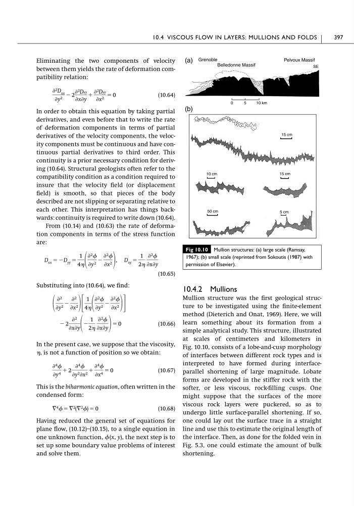
Fig. 10.10, consists of a lobe-and-cusp morphology
of interfaces between different rock types and is
interpreted to have formed during interfaceparallel shortening of large magnitude. Lobate
forms are developed in the stiffer rock with the
softer, or less viscous, rock-filling cusps. One
might suppose that the surfaces of the more
viscous rock layers were puckered, so as to
undergo little surface-parallel shortening. If so,
one could lay out the surface trace in a straight
line and use this to estimate the original length of
the interface. Then, as done for the folded vein in
Fig. 5.3, one could estimate the amount of bulk
shortening.
10.4 VISCOUS FLOW IN LAYERS: MULLIONS AND FOLDS
397
Fig 10.10 Mullion structures: (a) large scale (Ramsay,
1967); (b) small scale (reprinted from Sokoutis (1987) with
permission of Elsevier).
Grenoble
Belledonne Massif
Pelvoux Massif
SE
0
5
10 km
15 cm
10 cm
15 cm
50 cm
5 cm
(a)
(b)
between them yields the rate of deformation compatibility relation:
(10.64)
In order to obtain this equation by taking partial
derivatives, and even before that to write the rate
of deformation components in terms of partial
derivatives of the velocity components, the velocity components must be continuous and have continuous partial derivatives to third order. This
continuity is a prior necessary condition for deriving (10.64). Structural geologists often refer to the
compatibility condition as a condition required to
insure that the velocity field (or displacement
field) is smooth, so that pieces of the body
described are not slipping or separating relative to
each other. This interpretation has things backwards: continuity is required to write down (10.64).
From (10.14) and (10.63) the rate of deformation components in terms of the stress function
are:
(10.65)
Substituting into (10.64), we find:
(10.66)
In the present case, we suppose that the viscosity,
, is not a function of position so we obtain:
(10.67)
This is the biharmonic equation, often written in the
condensed form:
(10.68)
Having reduced the general set of equations for
plane flow, (10.12)–(10.15), to a single equation in
one unknown function, (x, y), the next step is to
set up some boundary value problems of interest
and solve them.
ٌ 4 ϭ ٌ 2 (ٌ 2 ) ϭ 0
Ѩ 4
Ѩy 4 ϩ 2
Ѩ 4
Ѩy 2 Ѩx 2 ϩ
Ѩ 4
Ѩx 4 ϭ 0
Ϫ 2
Ѩ 2
ѨxѨy Ϫ
1
2
Ѩ 2
ѨxѨy ϭ 0
Ѩ 2
Ѩy 2 Ϫ
Ѩ 2
Ѩx 2 ΄
1
4
Ѩ 2
Ѩy 2 Ϫ
Ѩ 2
Ѩx 2 ΅
D xx ϭ ϪD yy ϭ
1
4
Ѩ 2
Ѩy 2 Ϫ
Ѩ 2
Ѩx 2
, D xy ϭ
1
2
Ѩ 2
ѨxѨy
Ѩ 2 D xx
Ѩy 2 Ϫ 2
Ѩ 2 Dxy
ѨxѨy
ϩ
Ѩ 2 Dyy
Ѩx 2 ϭ 0
10.4.2 Mullions
Mullion structure was the first geological structure to be investigated using the finite-element
method (Dieterich and Onat, 1969). Here, we will
learn something about its formation from a
simple analytical study. This structure, illustrated
at scales of centimeters and kilometers in
Fig. 10.10, consists of a lobe-and-cusp morphology
of interfaces between different rock types and is
interpreted to have formed during interfaceparallel shortening of large magnitude. Lobate
forms are developed in the stiffer rock with the
softer, or less viscous, rock-filling cusps. One
might suppose that the surfaces of the more
viscous rock layers were puckered, so as to
undergo little surface-parallel shortening. If so,
one could lay out the surface trace in a straight
line and use this to estimate the original length of
the interface. Then, as done for the folded vein in
Fig. 5.3, one could estimate the amount of bulk
shortening.
10.4 VISCOUS FLOW IN LAYERS: MULLIONS AND FOLDS
397
Fig 10.10 Mullion structures: (a) large scale (Ramsay,
1967); (b) small scale (reprinted from Sokoutis (1987) with
permission of Elsevier).
Grenoble
Belledonne Massif
Pelvoux Massif
SE
0
5
10 km
15 cm
10 cm
15 cm
50 cm
5 cm
(a)
(b)