

(10.60)
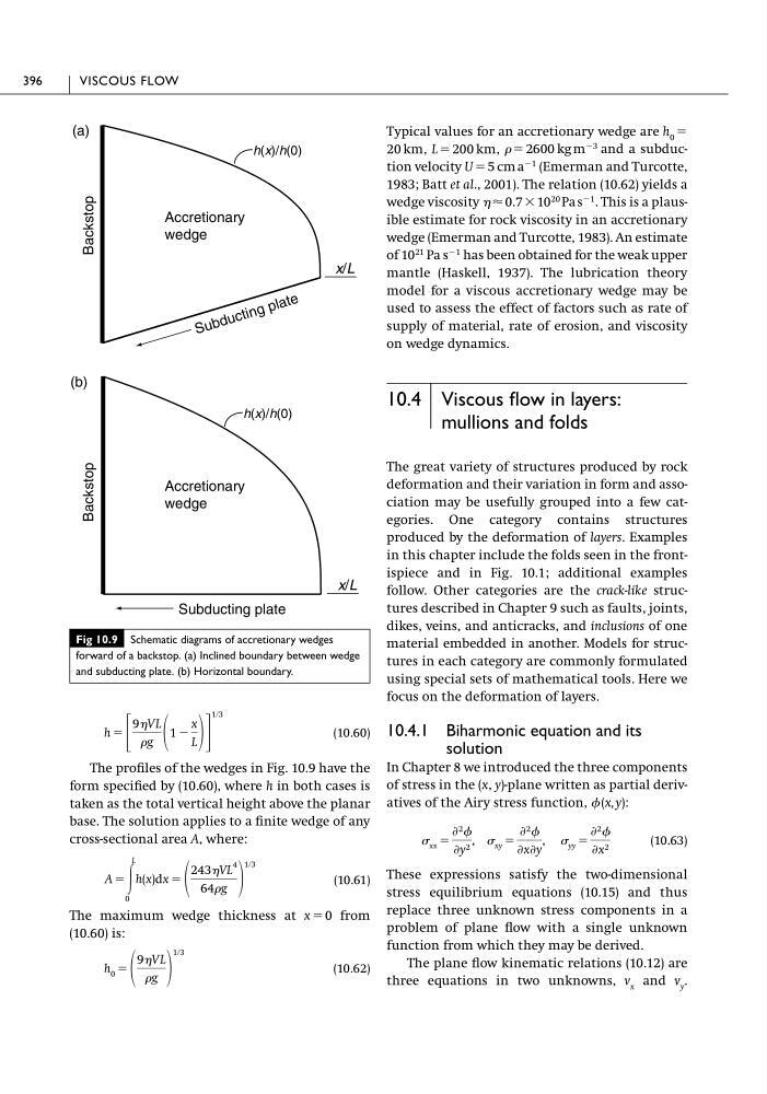
The profiles of the wedges in Fig. 10.9 have the
form specified by (10.60), where h in both cases is
taken as the total vertical height above the planar
base. The solution applies to a finite wedge of any
cross-sectional area A, where:
(10.61)
The maximum wedge thickness at x ϭ 0 from
(10.60) is:
(10.62)
h 0 ϭ
9VL
g
1ր3
A ϭ Ύ
L
0
h(x)dx ϭ
243VL
4
64g
1ր3
h ϭ ΄
9VL
g 1 Ϫ
x
L ΅
1ր3
Typical values for an accretionary wedge are h 0 ϭ
20 km, L ϭ 200 km, ϭ 2600 kg m
Ϫ3 and a subduction velocity U ϭ 5 cm a
Ϫ1 (Emerman and Turcotte,
1983; Batt et al., 2001). The relation (10.62) yields a
wedge viscosity Ϸ 0.7 ϫ 10
20 Pa s
Ϫ1 . This is a plausible estimate for rock viscosity in an accretionary
wedge (Emerman and Turcotte, 1983). An estimate
of 10
21 Pa s
Ϫ1 has been obtained for the weak upper
mantle (Haskell, 1937). The lubrication theory
model for a viscous accretionary wedge may be
used to assess the effect of factors such as rate of
supply of material, rate of erosion, and viscosity
on wedge dynamics.
10.4 Viscous flow in layers:
mullions and folds
The great variety of structures produced by rock
deformation and their variation in form and association may be usefully grouped into a few categories. One category contains structures
produced by the deformation of layers. Examples
in this chapter include the folds seen in the frontispiece and in Fig. 10.1; additional examples
follow. Other categories are the crack-like structures described in Chapter 9 such as faults, joints,
dikes, veins, and anticracks, and inclusions of one
material embedded in another. Models for structures in each category are commonly formulated
using special sets of mathematical tools. Here we
focus on the deformation of layers.
10.4.1 Biharmonic equation and its
solution
In Chapter 8 we introduced the three components
of stress in the (x, y)-plane written as partial derivatives of the Airy stress function, (x,y):
(10.63)
These expressions satisfy the two-dimensional
stress equilibrium equations (10.15) and thus
replace three unknown stress components in a
problem of plane flow with a single unknown
function from which they may be derived.
The plane flow kinematic relations (10.12) are
three equations in two unknowns, v x and v y .
xx ϭ
Ѩ 2
Ѩy 2 , xy ϭ
Ѩ 2
ѨxѨy
, yy ϭ
Ѩ 2
Ѩx 2
396
VISCOUS FLOW
Fig 10.9 Schematic diagrams of accretionary wedges
forward of a backstop. (a) Inclined boundary between wedge
and subducting plate. (b) Horizontal boundary.
(a)
(b)
S u b d u c ti n g p la te
Accretionary
wedge
x/L
Backstop
x/L
Backstop
Accretionary
wedge
Subducting plate
h(x)/h(0)
h(x)/h(0)
The profiles of the wedges in Fig. 10.9 have the
form specified by (10.60), where h in both cases is
taken as the total vertical height above the planar
base. The solution applies to a finite wedge of any
cross-sectional area A, where:
(10.61)
The maximum wedge thickness at x ϭ 0 from
(10.60) is:
(10.62)
h 0 ϭ
9VL
g
1ր3
A ϭ Ύ
L
0
h(x)dx ϭ
243VL
4
64g
1ր3
h ϭ ΄
9VL
g 1 Ϫ
x
L ΅
1ր3
Typical values for an accretionary wedge are h 0 ϭ
20 km, L ϭ 200 km, ϭ 2600 kg m
Ϫ3 and a subduction velocity U ϭ 5 cm a
Ϫ1 (Emerman and Turcotte,
1983; Batt et al., 2001). The relation (10.62) yields a
wedge viscosity Ϸ 0.7 ϫ 10
20 Pa s
Ϫ1 . This is a plausible estimate for rock viscosity in an accretionary
wedge (Emerman and Turcotte, 1983). An estimate
of 10
21 Pa s
Ϫ1 has been obtained for the weak upper
mantle (Haskell, 1937). The lubrication theory
model for a viscous accretionary wedge may be
used to assess the effect of factors such as rate of
supply of material, rate of erosion, and viscosity
on wedge dynamics.
10.4 Viscous flow in layers:
mullions and folds
The great variety of structures produced by rock
deformation and their variation in form and association may be usefully grouped into a few categories. One category contains structures
produced by the deformation of layers. Examples
in this chapter include the folds seen in the frontispiece and in Fig. 10.1; additional examples
follow. Other categories are the crack-like structures described in Chapter 9 such as faults, joints,
dikes, veins, and anticracks, and inclusions of one
material embedded in another. Models for structures in each category are commonly formulated
using special sets of mathematical tools. Here we
focus on the deformation of layers.
10.4.1 Biharmonic equation and its
solution
In Chapter 8 we introduced the three components
of stress in the (x, y)-plane written as partial derivatives of the Airy stress function, (x,y):
(10.63)
These expressions satisfy the two-dimensional
stress equilibrium equations (10.15) and thus
replace three unknown stress components in a
problem of plane flow with a single unknown
function from which they may be derived.
The plane flow kinematic relations (10.12) are
three equations in two unknowns, v x and v y .
xx ϭ
Ѩ 2
Ѩy 2 , xy ϭ
Ѩ 2
ѨxѨy
, yy ϭ
Ѩ 2
Ѩx 2
396
VISCOUS FLOW
Fig 10.9 Schematic diagrams of accretionary wedges
forward of a backstop. (a) Inclined boundary between wedge
and subducting plate. (b) Horizontal boundary.
(a)
(b)
S u b d u c ti n g p la te
Accretionary
wedge
x/L
Backstop
x/L
Backstop
Accretionary
wedge
Subducting plate
h(x)/h(0)
h(x)/h(0)