

The magnitude of the velocity of each plate is V.
We select the coordinate axes so that the flow will
have maximum symmetry:
(10.32)
That is, v x is an even function of y and an odd function of x, and v y is an odd function of y. The second
restriction implies that
A vertical
mirror plane of symmetry is present at x ϭ 0. Such
a plane behaves like the frictionless surface of
a rigid medium, preventing horizontal flow.
Symmetry also requires that the shear traction on
the (x ϭ 0)-plane be zero.
Fluid flows in opposite directions from the
central mirror plane of symmetry. The fluid flux
at some distance |x| from the mirror plane must
be equal to the volume per unit depth swept out
by the approaching plates per unit time, or 2V|x|.
Both conditions can be met by setting v x ϳ x. The
simplest function satisfying this condition and
(10.31) is:
(10.33)
From incompressibility the velocity gradients are
related as:
(10.34)
Integrating (10.34) we find:
(10.35)
This velocity distribution satisfies the conditions
(10.31) if:
(10.36)
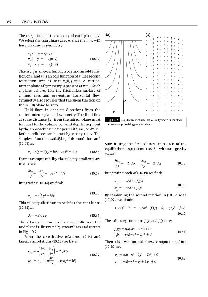
The velocity field over a distance of 4h from the
mid-plane is illustrated by streamlines and vectors
in Fig. 10.7.
From the constitutive relations (10.14) and
kinematic relations (10.12) we have:
(10.37)
xx Ϫ yy ϭ 4
Ѩv x
Ѩx
ϭ 4 A( y 2 Ϫ h 2 )
xy ϭ
Ѩv y
Ѩx
ϩ
Ѩv x
Ѩy
ϭ 2Axy
A ϭ Ϫ3Vր2h 3
v y ϭ ϪA(
1
3 y 3 Ϫ h 2 y)
Ѩv y
Ѩy
ϭ Ϫ
Ѩv x
Ѩx
ϭ ϪA( y 2 Ϫ h 2 )
v x ϭ A(y Ϫ h)( y ϩ h)x ϭ A( y 2 Ϫ h 2 )x
v x (0, y) ϭ 0.
v x (Ϫx, y) ϭ Ϫ v x (x, y)
v y (x,Ϫy) ϭ Ϫ v y (x, y)
v x (x,Ϫy) ϭ v x (x, y)
Substituting the first of these into each of the
equilibrium equations (10.15) without gravity
yields:
(10.38)
Integrating each of (10.38) we find:
(10.39)
By combining the second relation in (10.37) with
(10.39), we obtain:
(10.40)
The arbitrary functions f 1 (y) and f 2 (x) are:
(10.41)
Then the two normal stress components from
(10.39) are:
(10.42)
yy ϭ A(Ϫx 2 Ϫ y 2 ϩ 2h 2 ) ϩ C
xx ϭ A(Ϫx 2 ϩ 3y 2 Ϫ 2h 2 ) ϩ C
f 2 (x) ϭ A(Ϫx 2 ϩ 2h 2 ) ϩ C
f 1 ( y) ϭ A(3y 2 Ϫ 2h 2 ) ϩ C
4A( y 2 Ϫ h 2 ) ϭ Ϫ Ax 2 ϩ f 1 ( y) ϩ C 1 ϩ Ay 2 Ϫ f 2 (x)
yy ϭ Ϫ Ay 2 ϩ f 2 (x)
xx ϭ ϪAx 2 ϩ f 1 ( y)
Ѩ xx
Ѩx
ϭ Ϫ2 Ax,
Ѩ yy
Ѩy
ϭ Ϫ2 Ay
392
VISCOUS FLOW
Fig 10.7 (a) Streamlines and (b) velocity vectors for flow
between approaching parallel plates.
(a)
(b)
x
y
We select the coordinate axes so that the flow will
have maximum symmetry:
(10.32)
That is, v x is an even function of y and an odd function of x, and v y is an odd function of y. The second
restriction implies that
A vertical
mirror plane of symmetry is present at x ϭ 0. Such
a plane behaves like the frictionless surface of
a rigid medium, preventing horizontal flow.
Symmetry also requires that the shear traction on
the (x ϭ 0)-plane be zero.
Fluid flows in opposite directions from the
central mirror plane of symmetry. The fluid flux
at some distance |x| from the mirror plane must
be equal to the volume per unit depth swept out
by the approaching plates per unit time, or 2V|x|.
Both conditions can be met by setting v x ϳ x. The
simplest function satisfying this condition and
(10.31) is:
(10.33)
From incompressibility the velocity gradients are
related as:
(10.34)
Integrating (10.34) we find:
(10.35)
This velocity distribution satisfies the conditions
(10.31) if:
(10.36)
The velocity field over a distance of 4h from the
mid-plane is illustrated by streamlines and vectors
in Fig. 10.7.
From the constitutive relations (10.14) and
kinematic relations (10.12) we have:
(10.37)
xx Ϫ yy ϭ 4
Ѩv x
Ѩx
ϭ 4 A( y 2 Ϫ h 2 )
xy ϭ
Ѩv y
Ѩx
ϩ
Ѩv x
Ѩy
ϭ 2Axy
A ϭ Ϫ3Vր2h 3
v y ϭ ϪA(
1
3 y 3 Ϫ h 2 y)
Ѩv y
Ѩy
ϭ Ϫ
Ѩv x
Ѩx
ϭ ϪA( y 2 Ϫ h 2 )
v x ϭ A(y Ϫ h)( y ϩ h)x ϭ A( y 2 Ϫ h 2 )x
v x (0, y) ϭ 0.
v x (Ϫx, y) ϭ Ϫ v x (x, y)
v y (x,Ϫy) ϭ Ϫ v y (x, y)
v x (x,Ϫy) ϭ v x (x, y)
Substituting the first of these into each of the
equilibrium equations (10.15) without gravity
yields:
(10.38)
Integrating each of (10.38) we find:
(10.39)
By combining the second relation in (10.37) with
(10.39), we obtain:
(10.40)
The arbitrary functions f 1 (y) and f 2 (x) are:
(10.41)
Then the two normal stress components from
(10.39) are:
(10.42)
yy ϭ A(Ϫx 2 Ϫ y 2 ϩ 2h 2 ) ϩ C
xx ϭ A(Ϫx 2 ϩ 3y 2 Ϫ 2h 2 ) ϩ C
f 2 (x) ϭ A(Ϫx 2 ϩ 2h 2 ) ϩ C
f 1 ( y) ϭ A(3y 2 Ϫ 2h 2 ) ϩ C
4A( y 2 Ϫ h 2 ) ϭ Ϫ Ax 2 ϩ f 1 ( y) ϩ C 1 ϩ Ay 2 Ϫ f 2 (x)
yy ϭ Ϫ Ay 2 ϩ f 2 (x)
xx ϭ ϪAx 2 ϩ f 1 ( y)
Ѩ xx
Ѩx
ϭ Ϫ2 Ax,
Ѩ yy
Ѩy
ϭ Ϫ2 Ay
392
VISCOUS FLOW
Fig 10.7 (a) Streamlines and (b) velocity vectors for flow
between approaching parallel plates.
(a)
(b)
x
y