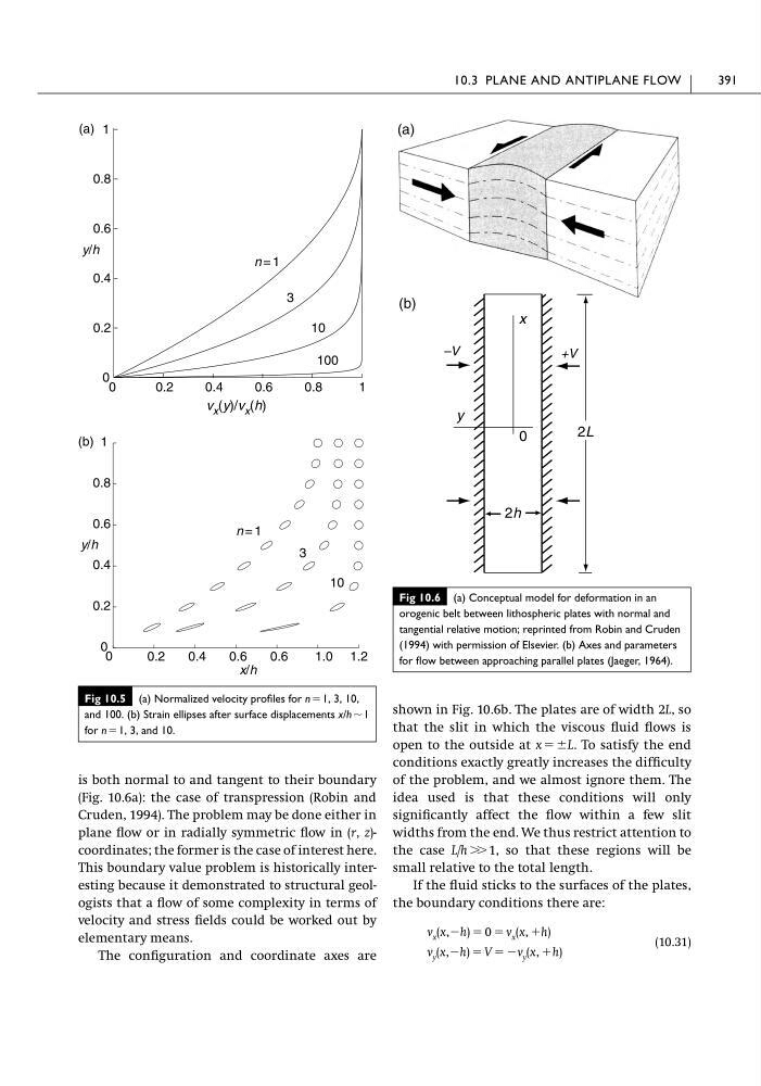
is both normal to and tangent to their boundary
(Fig. 10.6a): the case of transpression (Robin and
Cruden, 1994). The problem may be done either in
plane flow or in radially symmetric flow in (r, z)coordinates; the former is the case of interest here.
This boundary value problem is historically interesting because it demonstrated to structural geologists that a flow of some complexity in terms of
velocity and stress fields could be worked out by
elementary means.
The configuration and coordinate axes are
shown in Fig. 10.6b. The plates are of width 2L, so
that the slit in which the viscous fluid flows is
open to the outside at x ϭϮL. To satisfy the end
conditions exactly greatly increases the difficulty
of the problem, and we almost ignore them. The
idea used is that these conditions will only
significantly affect the flow within a few slit
widths from the end. We thus restrict attention to
the case L/h Ͼ Ͼ 1, so that these regions will be
small relative to the total length.
If the fluid sticks to the surfaces of the plates,
the boundary conditions there are:
(10.31)
v y (x,Ϫh) ϭ V ϭ Ϫv y (x, ϩh)
v x (x,Ϫh) ϭ 0 ϭ v x (x, ϩh)
10.3 PLANE AND ANTIPLANE FLOW
391
Fig 10.5 (a) Normalized velocity profiles for nϭ1, 3, 10,
and 100. (b) Strain ellipses after surface displacements x/hϳ1
for n ϭ 1, 3, and 10.
0
0.2
0.4
0.6
0.8
1
0
0.2
0.4
0.6
0.8
1
n = 1
3
10
100
y/h
v x (y)/v x (h)
(a)
0
0.2
0.4
0.6
0.6
1.0 1.2
0
0.2
0.4
0.6
0.8
1
y/h
x/h
n = 1
3
10
(b)
Fig 10.6 (a) Conceptual model for deformation in an
orogenic belt between lithospheric plates with normal and
tangential relative motion; reprinted from Robin and Cruden
(1994) with permission of Elsevier. (b) Axes and parameters
for flow between approaching parallel plates (Jaeger, 1964).
–V
+V
y
2h
x
0
(a)
2L
(b)