

The term in the first braces is the velocity at the
surface of the layer, y ϭ h, since the second term
equals 1 when y ϭ h. For given material properties,
n and B, one may evaluate this velocity. Alternatively, we may measure glacier thicknesses, slopes,
and surface velocities to estimate these properties, in the spirit of a field experiment. Notice that
the surface velocity is proportional to h
nϩ 1 .
An effect of the stress exponent, n, may be seen
by plotting the dimensionless ratio v x /v x (h) against
y/h for various n (Fig. 10.5a). As n increases, shearing becomes strongly concentrated downward
with increasing shear stress. For example, velocity
profiles through the thickness of a glacier may be
measured by melting a vertical borehole and
placing a cable in it (Raymond, 1971; Meier et al.,
1974). After an interval of time, the cable may be
“re-occupied” by sliding a melting device along it.
Measurement of the inclination of the cable as a
function of inextensible wire length from the
surface then allows the profile to be determined
by integration from the surface position.
If a mass of rock did flow in approximately
this fashion, and was cut by erosion, measurement of the shear strain distribution would allow
one to estimate n. Given the velocity field, which
in this case is steady, we may determine the distribution of strain in the body for a given amount
of surface displacement (Fig. 10.5b). Total displacement is different for each profile in order to
separate them. The deformed shapes of small
circles initially situated along the y/h-axis were
computed from a series of initial particle positions. Because of the gradient in shear rate, the
resulting loci only approximate ellipses. For
example, see the strongly deformed circle at the
base of the sheet for n ϭ 10. Procedures in Chapter
5 provide exact results: since the velocity gradient tensor for a particle is constant as it moves
along a line at constant height y, the displacement gradient tensor may be computed by direct
integration.
10.3.3 Flow between approaching or
separating rigid plates
The flow of fluid outward from approaching rigid
plates has been in the literature of structural
geology for several decades (Jaeger, 1964a). It has
been applied to deformation in an orogenic belt
between lithospheric plates whose relative motion
390
VISCOUS FLOW
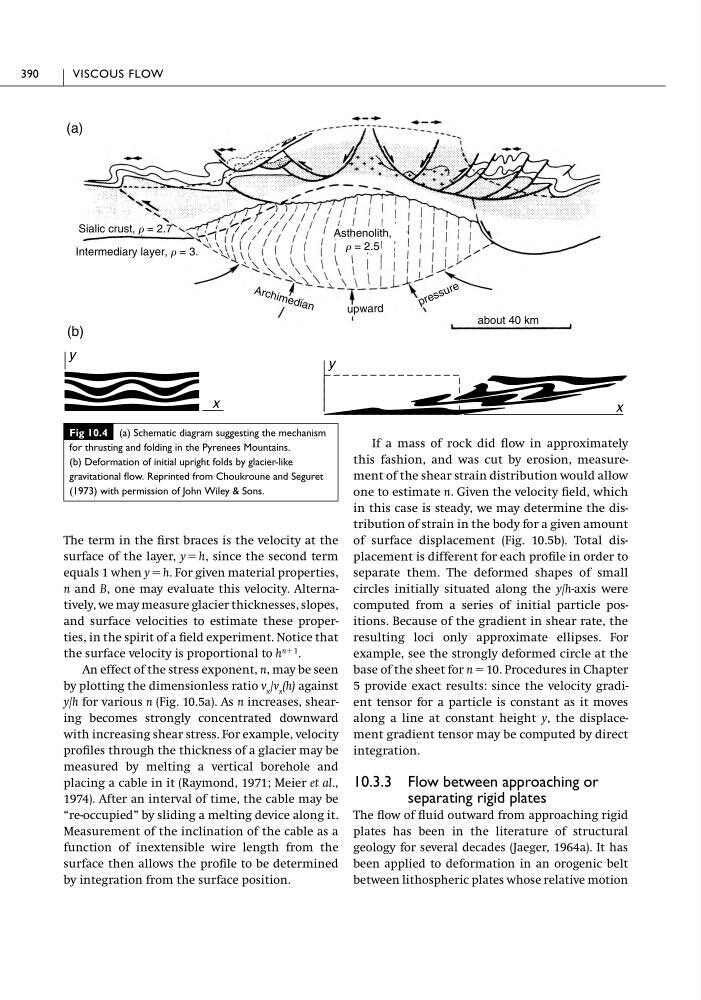
Fig 10.4 (a) Schematic diagram suggesting the mechanism
for thrusting and folding in the Pyrenees Mountains.
(b) Deformation of initial upright folds by glacier-like
gravitational flow. Reprinted from Choukroune and Seguret
(1973) with permission of John Wiley & Sons.
x
x
y
y
(a)
(b)
about 40 km
Asthenolith,
r = 2.5
Intermediary layer, r = 3.
Sialic crust, r = 2.7
A rc h im e d ia n
upward
p r e s s u r e
surface of the layer, y ϭ h, since the second term
equals 1 when y ϭ h. For given material properties,
n and B, one may evaluate this velocity. Alternatively, we may measure glacier thicknesses, slopes,
and surface velocities to estimate these properties, in the spirit of a field experiment. Notice that
the surface velocity is proportional to h
nϩ 1 .
An effect of the stress exponent, n, may be seen
by plotting the dimensionless ratio v x /v x (h) against
y/h for various n (Fig. 10.5a). As n increases, shearing becomes strongly concentrated downward
with increasing shear stress. For example, velocity
profiles through the thickness of a glacier may be
measured by melting a vertical borehole and
placing a cable in it (Raymond, 1971; Meier et al.,
1974). After an interval of time, the cable may be
“re-occupied” by sliding a melting device along it.
Measurement of the inclination of the cable as a
function of inextensible wire length from the
surface then allows the profile to be determined
by integration from the surface position.
If a mass of rock did flow in approximately
this fashion, and was cut by erosion, measurement of the shear strain distribution would allow
one to estimate n. Given the velocity field, which
in this case is steady, we may determine the distribution of strain in the body for a given amount
of surface displacement (Fig. 10.5b). Total displacement is different for each profile in order to
separate them. The deformed shapes of small
circles initially situated along the y/h-axis were
computed from a series of initial particle positions. Because of the gradient in shear rate, the
resulting loci only approximate ellipses. For
example, see the strongly deformed circle at the
base of the sheet for n ϭ 10. Procedures in Chapter
5 provide exact results: since the velocity gradient tensor for a particle is constant as it moves
along a line at constant height y, the displacement gradient tensor may be computed by direct
integration.
10.3.3 Flow between approaching or
separating rigid plates
The flow of fluid outward from approaching rigid
plates has been in the literature of structural
geology for several decades (Jaeger, 1964a). It has
been applied to deformation in an orogenic belt
between lithospheric plates whose relative motion
390
VISCOUS FLOW
Fig 10.4 (a) Schematic diagram suggesting the mechanism
for thrusting and folding in the Pyrenees Mountains.
(b) Deformation of initial upright folds by glacier-like
gravitational flow. Reprinted from Choukroune and Seguret
(1973) with permission of John Wiley & Sons.
x
x
y
y
(a)
(b)
about 40 km
Asthenolith,
r = 2.5
Intermediary layer, r = 3.
Sialic crust, r = 2.7
A rc h im e d ia n
upward
p r e s s u r e