

(9.48)
Note that the critical Coulomb stress is a function
of the coefficient of internal friction, half the
principal stress difference (equivalent to the
maximum shearing stress), and half the principal
stress sum (equivalent to the mean normal stress
in the plane of interest). As before one may use
the effective principal stresses,
to account for pore fluid
pressure.
The inherent shear strength is defined as the
critical Coulomb stress reaching a limiting value:
(9.49)
This relationship is useful in analyses where the
state of stress is computed using the solution to a
boundary value problem. Given the principal
stresses at these points, the coefficient of internal
friction, and the inherent shear strength, one can
use (9.48) to compute the normalized critical
Coulomb stress, CC /S 0 , over the region of interest.
Failure is predicted when this quantity equals
one. By computing the orientations of the principal stresses and using (9.45), one can predict the
orientations of the potential shear fractures. Then
CC /S 0 is contoured over the region of interest,
thereby identifying the areas most prone to shear
failure. This methodology was developed by
Hubbert (1951) and Hafner (1951), and many
others have followed their example for analyzing
the state of stress in Earth’s crust and the development of faults using the Coulomb criterion
(Sanford, 1959; Couples, 1977; Segall and Pollard,
1980; Bourne and Willemse, 2001; Crider, 2001;
Guiton et al., 2003).
It should be emphasized that the stress state
will change as soon as the first fault initiates. To
continue the analysis one must resort to numerical solutions of the boundary value problem in
which the fault is explicitly included as a surface
of displacement discontinuity. An example was
described in Chapter 1 for normal faults from the
Oseberg Field of the North Sea (Fig. 1.10)
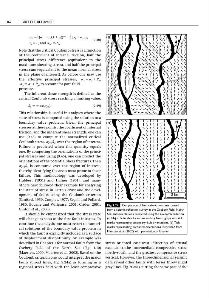
(Maerten, 2000; Maerten et al., 2002). Based on the
Coulomb criterion one would interpret the major
faults (broad lines, Fig. 9.24a) as forming in a
regional stress field with the least compressive
S 0 ϵ max ( CC ),
Ј 3 ϭ 3 ϩ P p ,
Ј 1 ϭ 1 ϩ P p ,
1 Ͻ T u and CC Յ S 0
CC ϭ
1
2 ( 1 Ϫ 3 )(1 ϩ 2
i ) 1ր2 ϩ
1
2 ( 1 ϩ 3 ) i
stress oriented east–west (direction of crustal
extension), the intermediate compressive stress
north–south, and the greatest compressive stress
vertical. However, the three-dimensional seismic
data reveal other faults with lesser throw (light
gray lines, Fig. 9.24a) cutting the same part of the
362
BRITTLE BEHAVIOR
Fig 9.24 Comparison of fault orientations interpreted
from a seismic reflection survey in the Oseberg Field, North
Sea, and orientations predicted using the Coulomb criterion.
(a) Major faults (black) and secondary faults (gray) with tick
marks representing secondary fault orientations. (b) Tick
marks representing predicted orientations. Reprinted from
Maerten et al. (2002) with permission of Elsevier.
(a)
(b)
2 km
N
N
Note that the critical Coulomb stress is a function
of the coefficient of internal friction, half the
principal stress difference (equivalent to the
maximum shearing stress), and half the principal
stress sum (equivalent to the mean normal stress
in the plane of interest). As before one may use
the effective principal stresses,
to account for pore fluid
pressure.
The inherent shear strength is defined as the
critical Coulomb stress reaching a limiting value:
(9.49)
This relationship is useful in analyses where the
state of stress is computed using the solution to a
boundary value problem. Given the principal
stresses at these points, the coefficient of internal
friction, and the inherent shear strength, one can
use (9.48) to compute the normalized critical
Coulomb stress, CC /S 0 , over the region of interest.
Failure is predicted when this quantity equals
one. By computing the orientations of the principal stresses and using (9.45), one can predict the
orientations of the potential shear fractures. Then
CC /S 0 is contoured over the region of interest,
thereby identifying the areas most prone to shear
failure. This methodology was developed by
Hubbert (1951) and Hafner (1951), and many
others have followed their example for analyzing
the state of stress in Earth’s crust and the development of faults using the Coulomb criterion
(Sanford, 1959; Couples, 1977; Segall and Pollard,
1980; Bourne and Willemse, 2001; Crider, 2001;
Guiton et al., 2003).
It should be emphasized that the stress state
will change as soon as the first fault initiates. To
continue the analysis one must resort to numerical solutions of the boundary value problem in
which the fault is explicitly included as a surface
of displacement discontinuity. An example was
described in Chapter 1 for normal faults from the
Oseberg Field of the North Sea (Fig. 1.10)
(Maerten, 2000; Maerten et al., 2002). Based on the
Coulomb criterion one would interpret the major
faults (broad lines, Fig. 9.24a) as forming in a
regional stress field with the least compressive
S 0 ϵ max ( CC ),
Ј 3 ϭ 3 ϩ P p ,
Ј 1 ϭ 1 ϩ P p ,
1 Ͻ T u and CC Յ S 0
CC ϭ
1
2 ( 1 Ϫ 3 )(1 ϩ 2
i ) 1ր2 ϩ
1
2 ( 1 ϩ 3 ) i
stress oriented east–west (direction of crustal
extension), the intermediate compressive stress
north–south, and the greatest compressive stress
vertical. However, the three-dimensional seismic
data reveal other faults with lesser throw (light
gray lines, Fig. 9.24a) cutting the same part of the
362
BRITTLE BEHAVIOR
Fig 9.24 Comparison of fault orientations interpreted
from a seismic reflection survey in the Oseberg Field, North
Sea, and orientations predicted using the Coulomb criterion.
(a) Major faults (black) and secondary faults (gray) with tick
marks representing secondary fault orientations. (b) Tick
marks representing predicted orientations. Reprinted from
Maerten et al. (2002) with permission of Elsevier.
(a)
(b)
2 km
N
N