

sedimentary sequence and trending oblique to
the major faults. It was hypothesized that these
faults developed in the same regional stress field,
but slip on the major faults locally perturbed this
field causing the smaller faults to form in oblique
orientations. To test this hypothesis the geometry
of the major faults was used as input for an
elastic model. When subjected to an east–west
extension the model faults slipped and the orientations of the principal stresses where computed. A comparison of the strikes of smaller
faults interpreted from the seismic survey and
the calculated directions of intermediate principal stress (Fig. 9.24b) suggests that the Coulomb
criterion provides a good correlation at many
locations.
9.3.3 The Coulomb criterion as a failure
surface in stress space
Failure in tension and in shear may be defined
using plots of a failure surface in principal stress
space based on theoretical criteria and these may
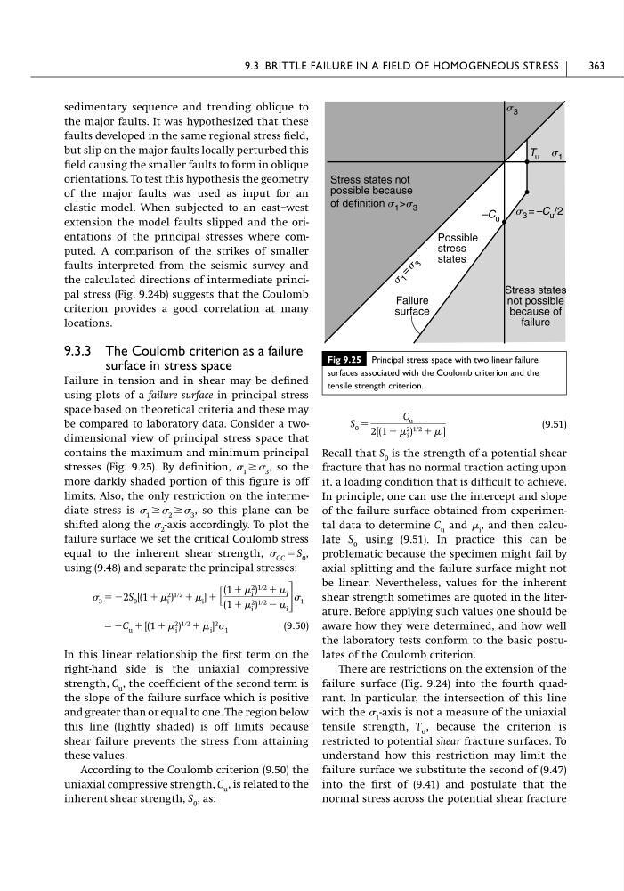
be compared to laboratory data. Consider a twodimensional view of principal stress space that
contains the maximum and minimum principal
stresses (Fig. 9.25). By definition, 1 Ն 3 , so the
more darkly shaded portion of this figure is off
limits. Also, the only restriction on the intermediate stress is 1 Ն 2 Ն 3 , so this plane can be
shifted along the 2 -axis accordingly. To plot the
failure surface we set the critical Coulomb stress
equal to the inherent shear strength, CC ϭ S 0 ,
using (9.48) and separate the principal stresses:
(9.50)
In this linear relationship the first term on the
right-hand side is the uniaxial compressive
strength, C u , the coefficient of the second term is
the slope of the failure surface which is positive
and greater than or equal to one. The region below
this line (lightly shaded) is off limits because
shear failure prevents the stress from attaining
these values.
According to the Coulomb criterion (9.50) the
uniaxial compressive strength, C u , is related to the
inherent shear strength, S 0 , as:
ϭ ϪC u ϩ [(1 ϩ 2
i ) 1ր2 ϩ i ] 2 1
3 ϭ Ϫ2S 0 [(1 ϩ 2
i ) 1ր2 ϩ i ] ϩ ΄
(1 ϩ 2
i ) 1ր2 ϩ i
(1 ϩ 2
i ) 1ր2 Ϫ i ΅ 1
(9.51)
Recall that S 0 is the strength of a potential shear
fracture that has no normal traction acting upon
it, a loading condition that is difficult to achieve.
In principle, one can use the intercept and slope
of the failure surface obtained from experimental data to determine C u and i , and then calculate S 0 using (9.51). In practice this can be
problematic because the specimen might fail by
axial splitting and the failure surface might not
be linear. Nevertheless, values for the inherent
shear strength sometimes are quoted in the literature. Before applying such values one should be
aware how they were determined, and how well
the laboratory tests conform to the basic postulates of the Coulomb criterion.
There are restrictions on the extension of the
failure surface (Fig. 9.24) into the fourth quadrant. In particular, the intersection of this line
with the 1 -axis is not a measure of the uniaxial
tensile strength, T u , because the criterion is
restricted to potential shear fracture surfaces. To
understand how this restriction may limit the
failure surface we substitute the second of (9.47)
into the first of (9.41) and postulate that the
normal stress across the potential shear fracture
S 0 ϭ
C u
2[(1 ϩ 2
i ) 1ր2 ϩ i ]
9.3 BRITTLE FAILURE IN A FIELD OF HOMOGENEOUS STRESS
363
Fig 9.25 Principal stress space with two linear failure
surfaces associated with the Coulomb criterion and the
tensile strength criterion.
–C u
s 3
Possible
stress
states
Stress states not
possible because
of definition s 1 >s 3
T u s 1
s 3 = –C u /2
s
1
=
s
3
Failure
surface
Stress states
not possible
because of
failure
the major faults. It was hypothesized that these
faults developed in the same regional stress field,
but slip on the major faults locally perturbed this
field causing the smaller faults to form in oblique
orientations. To test this hypothesis the geometry
of the major faults was used as input for an
elastic model. When subjected to an east–west
extension the model faults slipped and the orientations of the principal stresses where computed. A comparison of the strikes of smaller
faults interpreted from the seismic survey and
the calculated directions of intermediate principal stress (Fig. 9.24b) suggests that the Coulomb
criterion provides a good correlation at many
locations.
9.3.3 The Coulomb criterion as a failure
surface in stress space
Failure in tension and in shear may be defined
using plots of a failure surface in principal stress
space based on theoretical criteria and these may
be compared to laboratory data. Consider a twodimensional view of principal stress space that
contains the maximum and minimum principal
stresses (Fig. 9.25). By definition, 1 Ն 3 , so the
more darkly shaded portion of this figure is off
limits. Also, the only restriction on the intermediate stress is 1 Ն 2 Ն 3 , so this plane can be
shifted along the 2 -axis accordingly. To plot the
failure surface we set the critical Coulomb stress
equal to the inherent shear strength, CC ϭ S 0 ,
using (9.48) and separate the principal stresses:
(9.50)
In this linear relationship the first term on the
right-hand side is the uniaxial compressive
strength, C u , the coefficient of the second term is
the slope of the failure surface which is positive
and greater than or equal to one. The region below
this line (lightly shaded) is off limits because
shear failure prevents the stress from attaining
these values.
According to the Coulomb criterion (9.50) the
uniaxial compressive strength, C u , is related to the
inherent shear strength, S 0 , as:
ϭ ϪC u ϩ [(1 ϩ 2
i ) 1ր2 ϩ i ] 2 1
3 ϭ Ϫ2S 0 [(1 ϩ 2
i ) 1ր2 ϩ i ] ϩ ΄
(1 ϩ 2
i ) 1ր2 ϩ i
(1 ϩ 2
i ) 1ր2 Ϫ i ΅ 1
(9.51)
Recall that S 0 is the strength of a potential shear
fracture that has no normal traction acting upon
it, a loading condition that is difficult to achieve.
In principle, one can use the intercept and slope
of the failure surface obtained from experimental data to determine C u and i , and then calculate S 0 using (9.51). In practice this can be
problematic because the specimen might fail by
axial splitting and the failure surface might not
be linear. Nevertheless, values for the inherent
shear strength sometimes are quoted in the literature. Before applying such values one should be
aware how they were determined, and how well
the laboratory tests conform to the basic postulates of the Coulomb criterion.
There are restrictions on the extension of the
failure surface (Fig. 9.24) into the fourth quadrant. In particular, the intersection of this line
with the 1 -axis is not a measure of the uniaxial
tensile strength, T u , because the criterion is
restricted to potential shear fracture surfaces. To
understand how this restriction may limit the
failure surface we substitute the second of (9.47)
into the first of (9.41) and postulate that the
normal stress across the potential shear fracture
S 0 ϭ
C u
2[(1 ϩ 2
i ) 1ր2 ϩ i ]
9.3 BRITTLE FAILURE IN A FIELD OF HOMOGENEOUS STRESS
363
Fig 9.25 Principal stress space with two linear failure
surfaces associated with the Coulomb criterion and the
tensile strength criterion.
–C u
s 3
Possible
stress
states
Stress states not
possible because
of definition s 1 >s 3
T u s 1
s 3 = –C u /2
s
1
=
s
3
Failure
surface
Stress states
not possible
because of
failure