

of 3 km. The Coulomb stress was calculated by
solving the boundary value problem for an elastic
half-space with a fault that is 5.5 km long and 6 km
high with a maximum slip of 0.5 m tapering to
zero at the fault tip-lines. Two years of aftershock
locations are plotted on the same map and show
a distinct correlation to regions of elevated
Coulomb stress change. The locations and fault
plane solutions for earthquakes during the 1984
Morgan Hill seismic activity also show a correlation to Coulomb stress magnitudes and the
orientations of planes on which the maximum
Coulomb stress acts (Oppenheimer et al., 1988). The
locations of earthquakes that may have been triggered by the 1992 Landers earthquake also correlate with regions of elevated Coulomb stress (King
et al., 1994). These and other examples demonstrate the efficacy of this criterion for interpreting
shear failure at crustal scales in regions of active
faulting.
To carry out these analyses the Coulomb stress
is evaluated in terms of the maximum and
minimum principal stresses, 1 and 3 , rather
than the shear and normal components acting on
the potential shear fracture. This is done employing Cauchy’s Formula (6.55):
(9.41)
Here ␥ is the angle between the Ox-axis (here taken
parallel to the direction in which 1 acts) and the
normal, n, to the potential shear fracture (Fig.
9.21). Substituting these expressions into (9.40) we
have:
(9.42)
In order to proceed we exchange the absolute
value sign and the negative sign in the first term
on the right-hand side of this expression for a
Ϯ sign. Using these conditions (9.42) is written:
(9.43)
1 Ͻ T u and C Յ S 0
C ϭ
1
2 ( 1 Ϫ 3 )( Ϯ sin 2␥ ϩ i cos 2␥) ϩ
1
2 ( 1 ϩ 3 ) i
ϩ ΄
1
2 ( 1 ϩ 3 ) ϩ
1
2 ( 1 Ϫ 3 ) cos 2␥΅
C ϭ |Ϫ
1
2 ( 1 Ϫ 3 ) sin 2␥ |
s ϭ t s ϭ Ϫ
1
2 ( 1 Ϫ 3 ) sin 2␥
n ϭ t n ϭ
1
2 ( 1 ϩ 3 ) ϩ
1
2 ( 1 Ϫ 3 ) cos 2␥
The positive sign is used for ␥ in the first and third
quadrants and the negative sign is used for ␥ in
the second and fourth quadrants. This expression
is used to determine the Coulomb stress when one
knows (or postulates) the orientation, ␥, of the
potential shear fracture (Fig. 9.21), the coefficient
of internal friction, and the homogeneous stress
state in terms of the principal stresses or the effective principal stresses,
in the presence of pore fluids.
9.3.2 Predicting the orientation and
initiation of potential shear
fractures
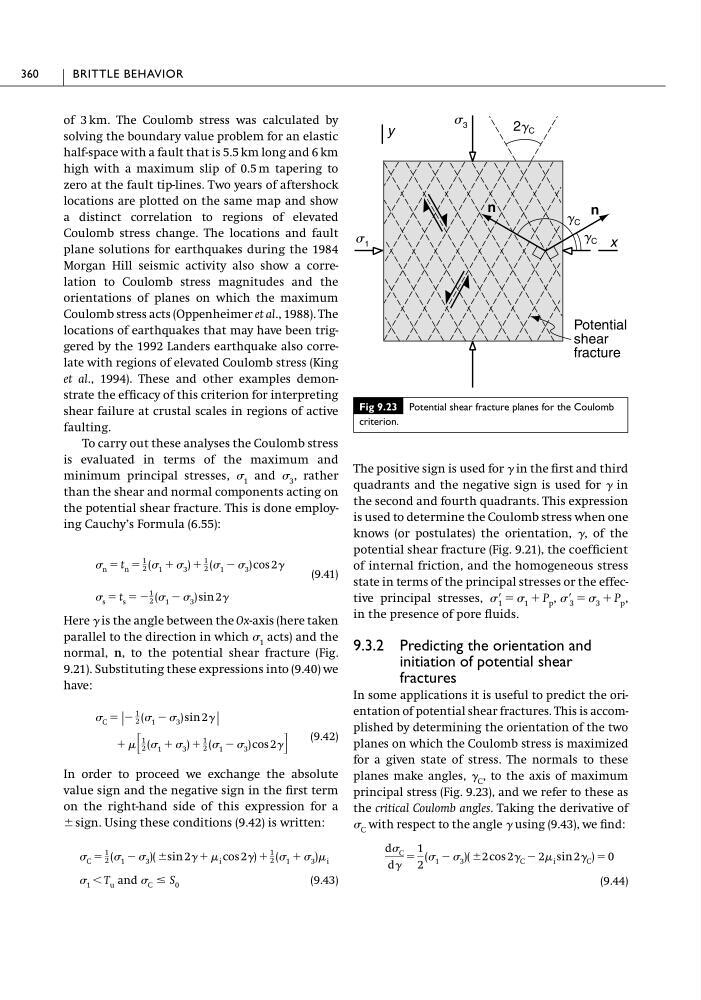
In some applications it is useful to predict the orientation of potential shear fractures. This is accomplished by determining the orientation of the two
planes on which the Coulomb stress is maximized
for a given state of stress. The normals to these
planes make angles, ␥ C , to the axis of maximum
principal stress (Fig. 9.23), and we refer to these as
the critical Coulomb angles. Taking the derivative of
C with respect to the angle ␥ using (9.43), we find:
(9.44)
d C
d␥
ϭ
1
2
( 1 Ϫ 3 )( Ϯ2 cos 2␥ C Ϫ 2 i sin 2␥ C ) ϭ 0
Ј 1 ϭ 1 ϩ P p , Ј 3 ϭ 3 ϩ P p ,
360
BRITTLE BEHAVIOR
Fig 9.23 Potential shear fracture planes for the Coulomb
criterion.
Potential
shear
fracture
y
x
2g C
s 3
g C
s 1
n
n
g C
solving the boundary value problem for an elastic
half-space with a fault that is 5.5 km long and 6 km
high with a maximum slip of 0.5 m tapering to
zero at the fault tip-lines. Two years of aftershock
locations are plotted on the same map and show
a distinct correlation to regions of elevated
Coulomb stress change. The locations and fault
plane solutions for earthquakes during the 1984
Morgan Hill seismic activity also show a correlation to Coulomb stress magnitudes and the
orientations of planes on which the maximum
Coulomb stress acts (Oppenheimer et al., 1988). The
locations of earthquakes that may have been triggered by the 1992 Landers earthquake also correlate with regions of elevated Coulomb stress (King
et al., 1994). These and other examples demonstrate the efficacy of this criterion for interpreting
shear failure at crustal scales in regions of active
faulting.
To carry out these analyses the Coulomb stress
is evaluated in terms of the maximum and
minimum principal stresses, 1 and 3 , rather
than the shear and normal components acting on
the potential shear fracture. This is done employing Cauchy’s Formula (6.55):
(9.41)
Here ␥ is the angle between the Ox-axis (here taken
parallel to the direction in which 1 acts) and the
normal, n, to the potential shear fracture (Fig.
9.21). Substituting these expressions into (9.40) we
have:
(9.42)
In order to proceed we exchange the absolute
value sign and the negative sign in the first term
on the right-hand side of this expression for a
Ϯ sign. Using these conditions (9.42) is written:
(9.43)
1 Ͻ T u and C Յ S 0
C ϭ
1
2 ( 1 Ϫ 3 )( Ϯ sin 2␥ ϩ i cos 2␥) ϩ
1
2 ( 1 ϩ 3 ) i
ϩ ΄
1
2 ( 1 ϩ 3 ) ϩ
1
2 ( 1 Ϫ 3 ) cos 2␥΅
C ϭ |Ϫ
1
2 ( 1 Ϫ 3 ) sin 2␥ |
s ϭ t s ϭ Ϫ
1
2 ( 1 Ϫ 3 ) sin 2␥
n ϭ t n ϭ
1
2 ( 1 ϩ 3 ) ϩ
1
2 ( 1 Ϫ 3 ) cos 2␥
The positive sign is used for ␥ in the first and third
quadrants and the negative sign is used for ␥ in
the second and fourth quadrants. This expression
is used to determine the Coulomb stress when one
knows (or postulates) the orientation, ␥, of the
potential shear fracture (Fig. 9.21), the coefficient
of internal friction, and the homogeneous stress
state in terms of the principal stresses or the effective principal stresses,
in the presence of pore fluids.
9.3.2 Predicting the orientation and
initiation of potential shear
fractures
In some applications it is useful to predict the orientation of potential shear fractures. This is accomplished by determining the orientation of the two
planes on which the Coulomb stress is maximized
for a given state of stress. The normals to these
planes make angles, ␥ C , to the axis of maximum
principal stress (Fig. 9.23), and we refer to these as
the critical Coulomb angles. Taking the derivative of
C with respect to the angle ␥ using (9.43), we find:
(9.44)
d C
d␥
ϭ
1
2
( 1 Ϫ 3 )( Ϯ2 cos 2␥ C Ϫ 2 i sin 2␥ C ) ϭ 0
Ј 1 ϭ 1 ϩ P p , Ј 3 ϭ 3 ϩ P p ,
360
BRITTLE BEHAVIOR
Fig 9.23 Potential shear fracture planes for the Coulomb
criterion.
Potential
shear
fracture
y
x
2g C
s 3
g C
s 1
n
n
g C