

The constant S 0 is referred to as the inherent shear
strength because this is the resistance to shear fracture when the normal stress is zero. Because shear
fractures develop independently of the sense of
shearing, the absolute value of the shear stress is
used. The effect of the normal stress is modified by
a constant, i , called the coefficient of internal friction. It should be understood that surfaces in frictional contact do not exist in the context of the
Coulomb criterion, so the name is misleading.
The linear relationship that relates shear and
normal traction components on sliding surfaces
is given by (9.30). The uniaxial tensile strength, T u ,
is used in (9.38) to restrict the stress state to those
that lead to shear fracture rather than tensile fracture. Because the actual stress state may be polyaxial, this restriction may have to include all
principal stresses and depend upon a more generalized tensile strength criterion (Bourne and
Willemse, 2001).
In (9.38) and what follows, the effective normal
stress,
may be substituted for the
normal stress to account for pore fluid pressure as
in (9.24):
(9.39)
Because the normal stress usually is compressive
(negative) and the pore pressure is a positive
number, the addition of pore pressure mitigates
the effect of the compression. In other words, the
greater the pore pressure the lesser the shear
stress required to induce shear fractures.
The Coulomb criterion (9.38) is used to define
the Coulomb stress, C :
(9.40)
The Coulomb stress may be used to compare different potential shear fracture orientations in a
deforming rock mass and assess which is closer to
failure. These could be differently oriented planes
at the same location subject to the same principal
stress state, or two planes at different locations
subject to different stress states. The potential
fracture surfaces could be in different rock types
with different coefficients of internal friction and
different pore pressures. In all cases the Coulomb
1 Ͻ T u and C Յ S 0
C ϭ | s | ϩ i n ,
1 Ͻ T u (shear fracture initiates)
| s | ϭ S 0 Ϫ i ( n ϩ P p ),
Ј n ϭ n ϩ P p ,
stress is viewed as the dependent variable and
would be calculated using the shear and normal
stress acting on the potential shear fracture
planes.
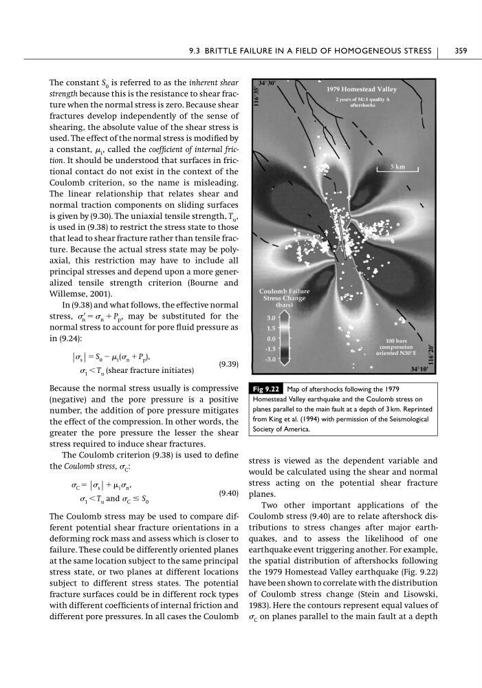
Two other important applications of the
Coulomb stress (9.40) are to relate aftershock distributions to stress changes after major earthquakes, and to assess the likelihood of one
earthquake event triggering another. For example,
the spatial distribution of aftershocks following
the 1979 Homestead Valley earthquake (Fig. 9.22)
have been shown to correlate with the distribution
of Coulomb stress change (Stein and Lisowski,
1983). Here the contours represent equal values of
C on planes parallel to the main fault at a depth
9.3 BRITTLE FAILURE IN A FIELD OF HOMOGENEOUS STRESS
359
Fig 9.22 Map of aftershocks following the 1979
Homestead Valley earthquake and the Coulomb stress on
planes parallel to the main fault at a depth of 3 km. Reprinted
from King et al. (1994) with permission of the Seismological
Society of America.
strength because this is the resistance to shear fracture when the normal stress is zero. Because shear
fractures develop independently of the sense of
shearing, the absolute value of the shear stress is
used. The effect of the normal stress is modified by
a constant, i , called the coefficient of internal friction. It should be understood that surfaces in frictional contact do not exist in the context of the
Coulomb criterion, so the name is misleading.
The linear relationship that relates shear and
normal traction components on sliding surfaces
is given by (9.30). The uniaxial tensile strength, T u ,
is used in (9.38) to restrict the stress state to those
that lead to shear fracture rather than tensile fracture. Because the actual stress state may be polyaxial, this restriction may have to include all
principal stresses and depend upon a more generalized tensile strength criterion (Bourne and
Willemse, 2001).
In (9.38) and what follows, the effective normal
stress,
may be substituted for the
normal stress to account for pore fluid pressure as
in (9.24):
(9.39)
Because the normal stress usually is compressive
(negative) and the pore pressure is a positive
number, the addition of pore pressure mitigates
the effect of the compression. In other words, the
greater the pore pressure the lesser the shear
stress required to induce shear fractures.
The Coulomb criterion (9.38) is used to define
the Coulomb stress, C :
(9.40)
The Coulomb stress may be used to compare different potential shear fracture orientations in a
deforming rock mass and assess which is closer to
failure. These could be differently oriented planes
at the same location subject to the same principal
stress state, or two planes at different locations
subject to different stress states. The potential
fracture surfaces could be in different rock types
with different coefficients of internal friction and
different pore pressures. In all cases the Coulomb
1 Ͻ T u and C Յ S 0
C ϭ | s | ϩ i n ,
1 Ͻ T u (shear fracture initiates)
| s | ϭ S 0 Ϫ i ( n ϩ P p ),
Ј n ϭ n ϩ P p ,
stress is viewed as the dependent variable and
would be calculated using the shear and normal
stress acting on the potential shear fracture
planes.
Two other important applications of the
Coulomb stress (9.40) are to relate aftershock distributions to stress changes after major earthquakes, and to assess the likelihood of one
earthquake event triggering another. For example,
the spatial distribution of aftershocks following
the 1979 Homestead Valley earthquake (Fig. 9.22)
have been shown to correlate with the distribution
of Coulomb stress change (Stein and Lisowski,
1983). Here the contours represent equal values of
C on planes parallel to the main fault at a depth
9.3 BRITTLE FAILURE IN A FIELD OF HOMOGENEOUS STRESS
359
Fig 9.22 Map of aftershocks following the 1979
Homestead Valley earthquake and the Coulomb stress on
planes parallel to the main fault at a depth of 3 km. Reprinted
from King et al. (1994) with permission of the Seismological
Society of America.