

confining pressure and pore pressure play in
determining rock strength under conditions of
brittle deformation.
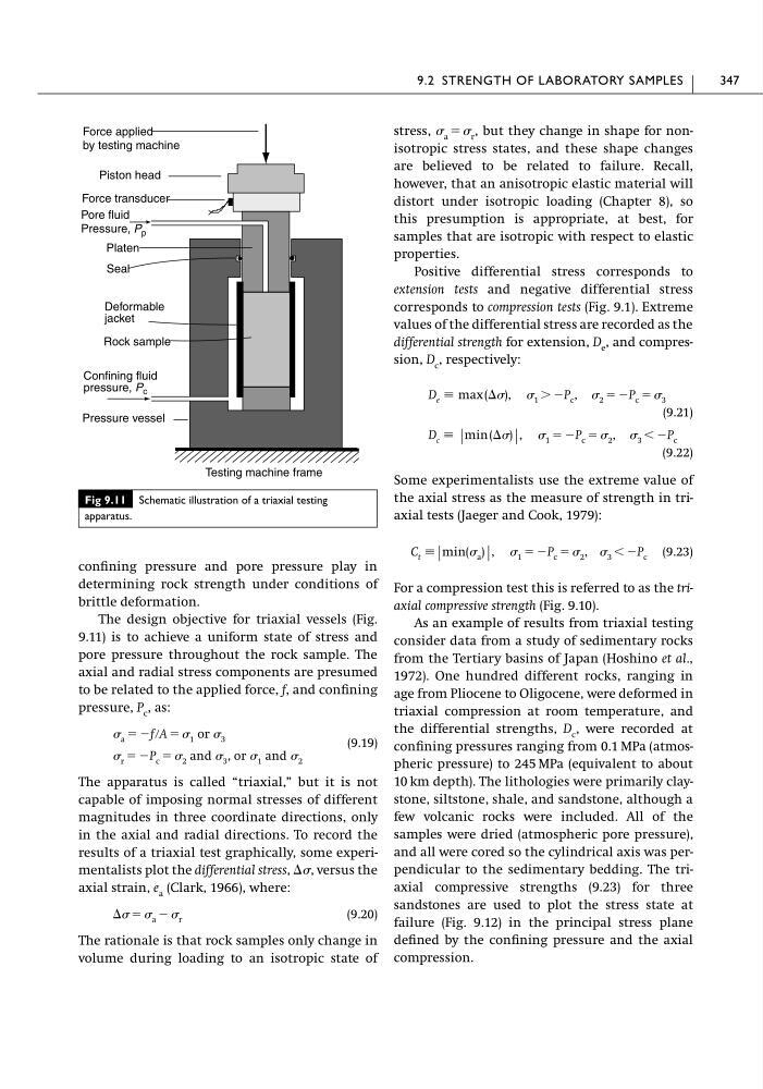
The design objective for triaxial vessels (Fig.
9.11) is to achieve a uniform state of stress and
pore pressure throughout the rock sample. The
axial and radial stress components are presumed
to be related to the applied force, f, and confining
pressure, P c , as:
(9.19)
The apparatus is called “triaxial,” but it is not
capable of imposing normal stresses of different
magnitudes in three coordinate directions, only
in the axial and radial directions. To record the
results of a triaxial test graphically, some experimentalists plot the differential stress, ⌬, versus the
axial strain, e a (Clark, 1966), where:
(9.20)
The rationale is that rock samples only change in
volume during loading to an isotropic state of
⌬ ϭ a Ϫ r
r ϭ ϪP c ϭ 2 and 3 , or 1 and 2
a ϭ Ϫf րA ϭ 1 or 3
stress, a ϭ r , but they change in shape for nonisotropic stress states, and these shape changes
are believed to be related to failure. Recall,
however, that an anisotropic elastic material will
distort under isotropic loading (Chapter 8), so
this presumption is appropriate, at best, for
samples that are isotropic with respect to elastic
properties.
Positive differential stress corresponds to
extension tests and negative differential stress
corresponds to compression tests (Fig. 9.1). Extreme
values of the differential stress are recorded as the
differential strength for extension, D e , and compression, D c , respectively:
(9.21)
(9.22)
Some experimentalists use the extreme value of
the axial stress as the measure of strength in triaxial tests (Jaeger and Cook, 1979):
(9.23)
For a compression test this is referred to as the triaxial compressive strength (Fig. 9.10).
As an example of results from triaxial testing
consider data from a study of sedimentary rocks
from the Tertiary basins of Japan (Hoshino et al.,
1972). One hundred different rocks, ranging in
age from Pliocene to Oligocene, were deformed in
triaxial compression at room temperature, and
the differential strengths, D c , were recorded at
confining pressures ranging from 0.1 MPa (atmospheric pressure) to 245 MPa (equivalent to about
10 km depth). The lithologies were primarily claystone, siltstone, shale, and sandstone, although a
few volcanic rocks were included. All of the
samples were dried (atmospheric pore pressure),
and all were cored so the cylindrical axis was perpendicular to the sedimentary bedding. The triaxial compressive strengths (9.23) for three
sandstones are used to plot the stress state at
failure (Fig. 9.12) in the principal stress plane
defined by the confining pressure and the axial
compression.
C t ϵ |min( a ) |, 1 ϭ ϪP c ϭ 2 , 3 Ͻ ϪP c
3 Ͻ ϪP c
D c ϵ |min (⌬) |, 1 ϭ ϪP c ϭ 2 ,
2 ϭ ϪP c ϭ 3
D e ϵ max (⌬), 1 Ͼ ϪP c ,
9.2 STRENGTH OF LABORATORY SAMPLES
347
Fig 9.11 Schematic illustration of a triaxial testing
apparatus.
Piston head
Force transducer
Rock sample
Pressure vessel
Pore fluid
Pressure, P p
Confining fluid
pressure, P c
Deformable
jacket
Seal
Force applied
by testing machine
Testing machine frame
Platen
determining rock strength under conditions of
brittle deformation.
The design objective for triaxial vessels (Fig.
9.11) is to achieve a uniform state of stress and
pore pressure throughout the rock sample. The
axial and radial stress components are presumed
to be related to the applied force, f, and confining
pressure, P c , as:
(9.19)
The apparatus is called “triaxial,” but it is not
capable of imposing normal stresses of different
magnitudes in three coordinate directions, only
in the axial and radial directions. To record the
results of a triaxial test graphically, some experimentalists plot the differential stress, ⌬, versus the
axial strain, e a (Clark, 1966), where:
(9.20)
The rationale is that rock samples only change in
volume during loading to an isotropic state of
⌬ ϭ a Ϫ r
r ϭ ϪP c ϭ 2 and 3 , or 1 and 2
a ϭ Ϫf րA ϭ 1 or 3
stress, a ϭ r , but they change in shape for nonisotropic stress states, and these shape changes
are believed to be related to failure. Recall,
however, that an anisotropic elastic material will
distort under isotropic loading (Chapter 8), so
this presumption is appropriate, at best, for
samples that are isotropic with respect to elastic
properties.
Positive differential stress corresponds to
extension tests and negative differential stress
corresponds to compression tests (Fig. 9.1). Extreme
values of the differential stress are recorded as the
differential strength for extension, D e , and compression, D c , respectively:
(9.21)
(9.22)
Some experimentalists use the extreme value of
the axial stress as the measure of strength in triaxial tests (Jaeger and Cook, 1979):
(9.23)
For a compression test this is referred to as the triaxial compressive strength (Fig. 9.10).
As an example of results from triaxial testing
consider data from a study of sedimentary rocks
from the Tertiary basins of Japan (Hoshino et al.,
1972). One hundred different rocks, ranging in
age from Pliocene to Oligocene, were deformed in
triaxial compression at room temperature, and
the differential strengths, D c , were recorded at
confining pressures ranging from 0.1 MPa (atmospheric pressure) to 245 MPa (equivalent to about
10 km depth). The lithologies were primarily claystone, siltstone, shale, and sandstone, although a
few volcanic rocks were included. All of the
samples were dried (atmospheric pore pressure),
and all were cored so the cylindrical axis was perpendicular to the sedimentary bedding. The triaxial compressive strengths (9.23) for three
sandstones are used to plot the stress state at
failure (Fig. 9.12) in the principal stress plane
defined by the confining pressure and the axial
compression.
C t ϵ |min( a ) |, 1 ϭ ϪP c ϭ 2 , 3 Ͻ ϪP c
3 Ͻ ϪP c
D c ϵ |min (⌬) |, 1 ϭ ϪP c ϭ 2 ,
2 ϭ ϪP c ϭ 3
D e ϵ max (⌬), 1 Ͼ ϪP c ,
9.2 STRENGTH OF LABORATORY SAMPLES
347
Fig 9.11 Schematic illustration of a triaxial testing
apparatus.
Piston head
Force transducer
Rock sample
Pressure vessel
Pore fluid
Pressure, P p
Confining fluid
pressure, P c
Deformable
jacket
Seal
Force applied
by testing machine
Testing machine frame
Platen