

samples may or may not be representative of the
strength in the natural setting of that rock, or of
the state that rock was in during the tectonic event
of interest to the structural geologist. Both the uniformity of the stress and the homogeneity of the
rock sample need to be evaluated when interpreting the results of laboratory strength tests. Finally,
the strength criteria (9.8) and (9.9) do not explicitly
address the physical mechanisms responsible for
the loss of load-carrying capacity; they simply
assert that this happens at a certain stress level.
9.2.3 Polyaxial strength, stress invariants,
and stress deviation
Below the traction-free surface of the Earth the
state of stress may be approximated by Anderson’s
standard state, introduced in Chapter 6, in which
the principal stresses are equal in magnitude
( 1 ϭ 2 ϭ 3 ) and become more compressive linearly with depth. This isotropic state of stress is
likely to be supplemented in regions of tectonic
activity by stresses that result in a polyaxial state of
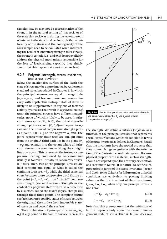
stress: the principal stresses have different magnitudes, none of which is likely to be zero. In principal stress space (Fig. 9.10), the uniaxial tensile
strength plots as a point (T u , 0, 0) on the positive 1 -
axis and the uniaxial compressive strength plots
as a point (0, 0, ϪC u ) on the negative 3 -axis. The
paths representing these tests are straight lines
from the origin. A third path lies in the plane ( 1
ϭ 2 ) and extends into the octant where all principal stresses are compressive along the straight
line 1 ϭ 2 ϭ 3 . This represents the isotropic compressive loading envisioned by Anderson and
usually is followed initially in laboratory “triaxial” tests. Then, two of the principal stresses are
held constant and equal to what is called the
confining pressure, ϪP c , while the third principal
stress becomes more compressive until failure at
the point (ϪP c , ϪP c , ϪC t ), the “triaxial” compressive strength (see next section). Strength in the
context of a polyaxial state of stress is represented
by a surface, called the failure surface, that passes
through these three points. The complete failure
surface separates possible states of stress between
the origin and the surface from impossible states
of stress on and beyond the surface.
The combination of principal stresses ( 1 , 2 ,
3 ) at any point on the failure surface represents
the strength. We define a criterion for failure as a
function of the principal stresses that represents
the failure surface and write this function in terms
of the stress invariants as defined in Chapter 6. Recall
that the invariants have the special property that
they do not change magnitude with the orientation of the Cartesian coordinate system. Because
physical properties of a material, such as strength,
should not depend upon the arbitrary orientation
of a coordinate system, it is natural to define such
properties in terms of the stress invariants (Jaeger
and Cook, 1979). Criteria for failure under uniaxial
conditions are equivalent to placing limiting
values on the first invariant of the stress tensor,
I 1 ϭ 1 ϩ 2 ϩ 3 , when only one principal stress is
non-zero:
(9.12)
(9.13)
Note that this pre-supposes that the initiation of
failure depends only upon the current homogeneous state of stress. That is, failure does not
I 1 ϭ ϪC 0 , 1 ϭ 0 ϭ 2
I 1 ϭ T 0 , 2 ϭ 0 ϭ 3
9.2 STRENGTH OF LABORATORY SAMPLES
345
Fig 9.10 Plot in principal stress space with uniaxial tensile
and compressive strengths, T u and C u , and triaxial
compressive strength, C t .
T u
s 2
s 1
s 3
s 1 = s 2 , s 3 = 0
s
1
= s
2
= s
3
–C u
–C t
s 1
= –P c
= s 2
strength in the natural setting of that rock, or of
the state that rock was in during the tectonic event
of interest to the structural geologist. Both the uniformity of the stress and the homogeneity of the
rock sample need to be evaluated when interpreting the results of laboratory strength tests. Finally,
the strength criteria (9.8) and (9.9) do not explicitly
address the physical mechanisms responsible for
the loss of load-carrying capacity; they simply
assert that this happens at a certain stress level.
9.2.3 Polyaxial strength, stress invariants,
and stress deviation
Below the traction-free surface of the Earth the
state of stress may be approximated by Anderson’s
standard state, introduced in Chapter 6, in which
the principal stresses are equal in magnitude
( 1 ϭ 2 ϭ 3 ) and become more compressive linearly with depth. This isotropic state of stress is
likely to be supplemented in regions of tectonic
activity by stresses that result in a polyaxial state of
stress: the principal stresses have different magnitudes, none of which is likely to be zero. In principal stress space (Fig. 9.10), the uniaxial tensile
strength plots as a point (T u , 0, 0) on the positive 1 -
axis and the uniaxial compressive strength plots
as a point (0, 0, ϪC u ) on the negative 3 -axis. The
paths representing these tests are straight lines
from the origin. A third path lies in the plane ( 1
ϭ 2 ) and extends into the octant where all principal stresses are compressive along the straight
line 1 ϭ 2 ϭ 3 . This represents the isotropic compressive loading envisioned by Anderson and
usually is followed initially in laboratory “triaxial” tests. Then, two of the principal stresses are
held constant and equal to what is called the
confining pressure, ϪP c , while the third principal
stress becomes more compressive until failure at
the point (ϪP c , ϪP c , ϪC t ), the “triaxial” compressive strength (see next section). Strength in the
context of a polyaxial state of stress is represented
by a surface, called the failure surface, that passes
through these three points. The complete failure
surface separates possible states of stress between
the origin and the surface from impossible states
of stress on and beyond the surface.
The combination of principal stresses ( 1 , 2 ,
3 ) at any point on the failure surface represents
the strength. We define a criterion for failure as a
function of the principal stresses that represents
the failure surface and write this function in terms
of the stress invariants as defined in Chapter 6. Recall
that the invariants have the special property that
they do not change magnitude with the orientation of the Cartesian coordinate system. Because
physical properties of a material, such as strength,
should not depend upon the arbitrary orientation
of a coordinate system, it is natural to define such
properties in terms of the stress invariants (Jaeger
and Cook, 1979). Criteria for failure under uniaxial
conditions are equivalent to placing limiting
values on the first invariant of the stress tensor,
I 1 ϭ 1 ϩ 2 ϩ 3 , when only one principal stress is
non-zero:
(9.12)
(9.13)
Note that this pre-supposes that the initiation of
failure depends only upon the current homogeneous state of stress. That is, failure does not
I 1 ϭ ϪC 0 , 1 ϭ 0 ϭ 2
I 1 ϭ T 0 , 2 ϭ 0 ϭ 3
9.2 STRENGTH OF LABORATORY SAMPLES
345
Fig 9.10 Plot in principal stress space with uniaxial tensile
and compressive strengths, T u and C u , and triaxial
compressive strength, C t .
T u
s 2
s 1
s 3
s 1 = s 2 , s 3 = 0
s
1
= s
2
= s
3
–C u
–C t
s 1
= –P c
= s 2