

(8.140)
Note that the sum and the product of the constants ␣ 1 and ␣ 2 are related to the compliances
(8.139), so one must solve these two equations
simultaneously to find these relations. Multiplying the second of (8.139) by ␣ 1 we have:
(8.141)
Subtracting the second equation from the first
equation we find the following quadratic equation:
(8.142)
The two solutions for this quadratic equation are:
(8.143)
The restriction on the values of C 1 and C 2 follows
from the fact that the compliances are real
numbers, so we are looking for solutions that are
real values of ␣ 1 , given real values of C 1 and C 2 .
These constants are related to the familiar elastic
constants as follows:
(8.144)
C 1 ϭ
s 11
s 22
ϭ
E 2
E 1
, C 2 ϭ
E 2
G
Ϫ 2 21
␣ 1 ϭ
1
2 C 2 Ϯ
1
2 √C 2
2 Ϫ 4C 1 , where C 2
2 Ϫ 4C 1 Ն 0
␣ 2
1 Ϫ C 2 ␣ 1 ϩ C 1 ϭ 0
␣ 1 ␣ 2 ϭ C 1 , ␣ 2
1 ϩ ␣ 1 ␣ 2 ϭ C 2 ␣ 1
Ѩ 2
Ѩx 2 ϩ ␣ 1
Ѩ 2
Ѩy 2
Ѩ 2
Ѩx 2 ϩ ␣ 2
Ѩ 2
Ѩy 2 ⌽ ϭ 0
For the purpose of illustrating the effects of
elastic anisotropy on the state of stress we consider the problem of the circular hole and select
the following values for the elastic constants: E 1 ϭ
40 GPa, E 2 ϭ20 GPa, G ϭ10 GPa, 12 ϭ0.2, 21 ϭ0.1.
This would be considered a very anisotropic rock,
judging from Table 8.6: the ratio E 1 /E 2 ϭ 2 is
greater than any of the examples given there. Only
four constants are independent and these five constants are self-consistent according to (8.133).
Using (8.144), we find C 1 ϭ 0.5 and C 2 ϭ 1.8, and
solving the quadratic equation (8.143) we have ␣ 1
ϭ (1.457, 0.343). Using the first of (8.141), the
second constant is ␣ 2 ϭ (0.343, 1.457). Note that
there is only one pair of independent constants
given by the solution to the quadratic equation.
This follows from (8.140) where one can see that
the constants ␣ 1 and ␣ 2 are interchangeable.
Stress states for the elastic boundary value
problem are given in terms of yet more constants
that are related to the constants ␣ 1 and ␣ 2 as
follows:
(8.145)
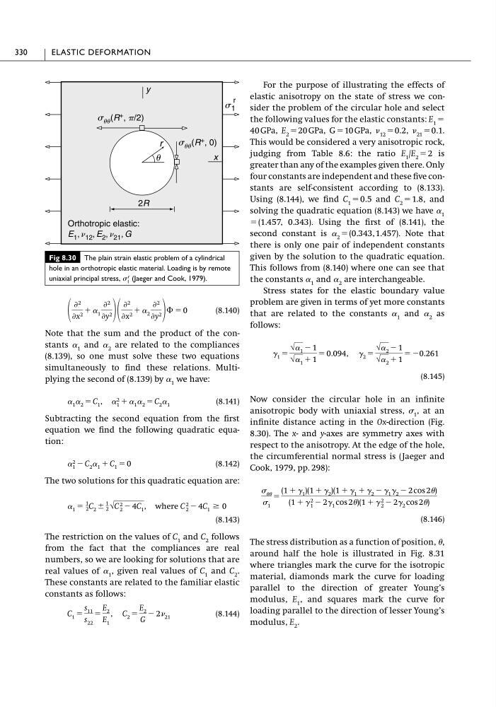
Now consider the circular hole in an infinite
anisotropic body with uniaxial stress, 1 , at an
infinite distance acting in the Ox-direction (Fig.
8.30). The x- and y-axes are symmetry axes with
respect to the anisotropy. At the edge of the hole,
the circumferential normal stress is (Jaeger and
Cook, 1979, pp. 298):
(8.146)
The stress distribution as a function of position, ,
around half the hole is illustrated in Fig. 8.31
where triangles mark the curve for the isotropic
material, diamonds mark the curve for loading
parallel to the direction of greater Young’s
modulus, E 1 , and squares mark the curve for
loading parallel to the direction of lesser Young’s
modulus, E 2 .
ϭ
(1 ϩ ␥ 1 )(1 ϩ ␥ 2 )(1 ϩ ␥ 1 ϩ ␥ 2 Ϫ ␥ 1 ␥ 2 Ϫ 2 cos 2)
(1 ϩ ␥ 2
1 Ϫ 2␥ 1 cos 2)(1 ϩ ␥ 2
2 Ϫ 2␥ 2 cos 2)
1
␥ 1 ϭ
√␣ 1 Ϫ 1
√␣ 1 ϩ 1
ϭ 0.094, ␥ 2 ϭ
√␣ 2 Ϫ 1
√␣ 2 ϩ 1
ϭ Ϫ0.261
330
ELASTIC DEFORMATION
Fig 8.30 The plain strain elastic problem of a cylindrical
hole in an orthotropic elastic material. Loading is by remote
uniaxial principal stress, 1
r (Jaeger and Cook, 1979).
y
x
2R
r
u
Orthotropic elastic:
E 1 , N 12 , E 2 , N 21 , G
s 1
r
s uu (R + , p/2)
s uu (R + , 0)
Note that the sum and the product of the constants ␣ 1 and ␣ 2 are related to the compliances
(8.139), so one must solve these two equations
simultaneously to find these relations. Multiplying the second of (8.139) by ␣ 1 we have:
(8.141)
Subtracting the second equation from the first
equation we find the following quadratic equation:
(8.142)
The two solutions for this quadratic equation are:
(8.143)
The restriction on the values of C 1 and C 2 follows
from the fact that the compliances are real
numbers, so we are looking for solutions that are
real values of ␣ 1 , given real values of C 1 and C 2 .
These constants are related to the familiar elastic
constants as follows:
(8.144)
C 1 ϭ
s 11
s 22
ϭ
E 2
E 1
, C 2 ϭ
E 2
G
Ϫ 2 21
␣ 1 ϭ
1
2 C 2 Ϯ
1
2 √C 2
2 Ϫ 4C 1 , where C 2
2 Ϫ 4C 1 Ն 0
␣ 2
1 Ϫ C 2 ␣ 1 ϩ C 1 ϭ 0
␣ 1 ␣ 2 ϭ C 1 , ␣ 2
1 ϩ ␣ 1 ␣ 2 ϭ C 2 ␣ 1
Ѩ 2
Ѩx 2 ϩ ␣ 1
Ѩ 2
Ѩy 2
Ѩ 2
Ѩx 2 ϩ ␣ 2
Ѩ 2
Ѩy 2 ⌽ ϭ 0
For the purpose of illustrating the effects of
elastic anisotropy on the state of stress we consider the problem of the circular hole and select
the following values for the elastic constants: E 1 ϭ
40 GPa, E 2 ϭ20 GPa, G ϭ10 GPa, 12 ϭ0.2, 21 ϭ0.1.
This would be considered a very anisotropic rock,
judging from Table 8.6: the ratio E 1 /E 2 ϭ 2 is
greater than any of the examples given there. Only
four constants are independent and these five constants are self-consistent according to (8.133).
Using (8.144), we find C 1 ϭ 0.5 and C 2 ϭ 1.8, and
solving the quadratic equation (8.143) we have ␣ 1
ϭ (1.457, 0.343). Using the first of (8.141), the
second constant is ␣ 2 ϭ (0.343, 1.457). Note that
there is only one pair of independent constants
given by the solution to the quadratic equation.
This follows from (8.140) where one can see that
the constants ␣ 1 and ␣ 2 are interchangeable.
Stress states for the elastic boundary value
problem are given in terms of yet more constants
that are related to the constants ␣ 1 and ␣ 2 as
follows:
(8.145)
Now consider the circular hole in an infinite
anisotropic body with uniaxial stress, 1 , at an
infinite distance acting in the Ox-direction (Fig.
8.30). The x- and y-axes are symmetry axes with
respect to the anisotropy. At the edge of the hole,
the circumferential normal stress is (Jaeger and
Cook, 1979, pp. 298):
(8.146)
The stress distribution as a function of position, ,
around half the hole is illustrated in Fig. 8.31
where triangles mark the curve for the isotropic
material, diamonds mark the curve for loading
parallel to the direction of greater Young’s
modulus, E 1 , and squares mark the curve for
loading parallel to the direction of lesser Young’s
modulus, E 2 .
ϭ
(1 ϩ ␥ 1 )(1 ϩ ␥ 2 )(1 ϩ ␥ 1 ϩ ␥ 2 Ϫ ␥ 1 ␥ 2 Ϫ 2 cos 2)
(1 ϩ ␥ 2
1 Ϫ 2␥ 1 cos 2)(1 ϩ ␥ 2
2 Ϫ 2␥ 2 cos 2)
1
␥ 1 ϭ
√␣ 1 Ϫ 1
√␣ 1 ϩ 1
ϭ 0.094, ␥ 2 ϭ
√␣ 2 Ϫ 1
√␣ 2 ϩ 1
ϭ Ϫ0.261
330
ELASTIC DEFORMATION
Fig 8.30 The plain strain elastic problem of a cylindrical
hole in an orthotropic elastic material. Loading is by remote
uniaxial principal stress, 1
r (Jaeger and Cook, 1979).
y
x
2R
r
u
Orthotropic elastic:
E 1 , N 12 , E 2 , N 21 , G
s 1
r
s uu (R + , p/2)
s uu (R + , 0)