

in contrast to the two elastic moduli for the
isotropic material (8.48)–(8.50) and define the socalled orthotropic solid:
(8.131)
In terms of Young’s moduli and Poisson’s ratios,
these equations are written:
(8.132)
What appear to be five constants are only four
because the two Poisson’s ratios are related:
(8.133)
E 1 and 12 are Young’s modulus and Poisson’s ratio
for an applied normal stress along the x-axis,
whereas E 2 and 21 are Young’s modulus and
Poisson’s ratio for an applied normal stress along
the y-axis. G is the shear modulus in the (x, y)plane.
For isotropic materials, the number of independent compliances reduces to two because:
(8.134)
How these compliances relate to the isotropic
elastic constants introduced earlier can be
deduced from the strain–stress relationships
written using the compliances and (8.134), and
comparing these to (8.18), (Nye, 1985, p. 143):
(8.135)
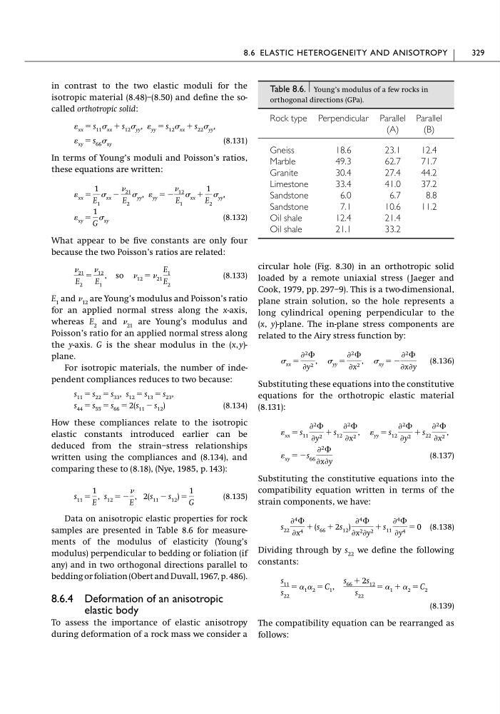
Data on anisotropic elastic properties for rock
samples are presented in Table 8.6 for measurements of the modulus of elasticity (Young’s
modulus) perpendicular to bedding or foliation (if
any) and in two orthogonal directions parallel to
bedding or foliation (Obert and Duvall, 1967, p. 486).
8.6.4 Deformation of an anisotropic
elastic body
To assess the importance of elastic anisotropy
during deformation of a rock mass we consider a
s 11 ϭ
1
E
, s 12 ϭ Ϫ
E
, 2(s 11 Ϫ s 12 ) ϭ
1
G
s 44 ϭ s 55 ϭ s 66 ϭ 2(s 11 Ϫ s 12 )
s 11 ϭ s 22 ϭ s 33 , s 12 ϭ s 13 ϭ s 23 ,
21
E 2
ϭ
12
E 1
, so 12 ϭ 21
E 1
E 2
xy ϭ
1
G
xy
xx ϭ
1
E 1
xx Ϫ
21
E 2
yy , yy ϭ Ϫ
12
E 1
xx ϩ
1
E 2
yy ,
xy ϭ s 66 xy
xx ϭ s 11 xx ϩ s 12 yy , yy ϭ s 12 xx ϩ s 22 yy ,
circular hole (Fig. 8.30) in an orthotropic solid
loaded by a remote uniaxial stress ( Jaeger and
Cook, 1979, pp. 297–9). This is a two-dimensional,
plane strain solution, so the hole represents a
long cylindrical opening perpendicular to the
(x, y)-plane. The in-plane stress components are
related to the Airy stress function by:
(8.136)
Substituting these equations into the constitutive
equations for the orthotropic elastic material
(8.131):
(8.137)
Substituting the constitutive equations into the
compatibility equation written in terms of the
strain components, we have:
(8.138)
Dividing through by s 22 we define the following
constants:
(8.139)
The compatibility equation can be rearranged as
follows:
s 11
s 22
ϭ ␣ 1 ␣ 2 ϭ C 1 ,
s 66 ϩ 2s 12
s 22
ϭ ␣ 1 ϩ ␣ 2 ϭ C 2
s 22
Ѩ 4 ⌽
Ѩx 4 ϩ (s 66 ϩ 2s 12 )
Ѩ 4 ⌽
Ѩx 2 Ѩy 2 ϩ s 11
Ѩ 4 ⌽
Ѩy 4 ϭ 0
xy ϭ Ϫs 66
Ѩ 2 ⌽
ѨxѨy
xx ϭ s 11
Ѩ 2 ⌽
Ѩy 2 ϩ s 12
Ѩ 2 ⌽
Ѩx 2 , yy ϭ s 12
Ѩ 2 ⌽
Ѩy 2 ϩ s 22
Ѩ 2 ⌽
Ѩx 2 ,
xx ϭ
Ѩ 2 ⌽
Ѩy 2 , yy ϭ
Ѩ 2 ⌽
Ѩx 2 , xy ϭ Ϫ
Ѩ 2 ⌽
ѨxѨy
8.6 ELASTIC HETEROGENEITY AND ANISOTROPY
329
Table 8.6. Young’s modulus of a few rocks in
orthogonal directions (GPa).
Rock type Perpendicular Parallel Parallel
(A)
(B)
Gneiss
18.6
23.1
12.4
Marble
49.3
62.7
71.7
Granite
30.4
27.4
44.2
Limestone
33.4
41.0
37.2
Sandstone
6.0
6.7
8.8
Sandstone
7.1
10.6
11.2
Oil shale
12.4
21.4
Oil shale
21.1
33.2
isotropic material (8.48)–(8.50) and define the socalled orthotropic solid:
(8.131)
In terms of Young’s moduli and Poisson’s ratios,
these equations are written:
(8.132)
What appear to be five constants are only four
because the two Poisson’s ratios are related:
(8.133)
E 1 and 12 are Young’s modulus and Poisson’s ratio
for an applied normal stress along the x-axis,
whereas E 2 and 21 are Young’s modulus and
Poisson’s ratio for an applied normal stress along
the y-axis. G is the shear modulus in the (x, y)plane.
For isotropic materials, the number of independent compliances reduces to two because:
(8.134)
How these compliances relate to the isotropic
elastic constants introduced earlier can be
deduced from the strain–stress relationships
written using the compliances and (8.134), and
comparing these to (8.18), (Nye, 1985, p. 143):
(8.135)
Data on anisotropic elastic properties for rock
samples are presented in Table 8.6 for measurements of the modulus of elasticity (Young’s
modulus) perpendicular to bedding or foliation (if
any) and in two orthogonal directions parallel to
bedding or foliation (Obert and Duvall, 1967, p. 486).
8.6.4 Deformation of an anisotropic
elastic body
To assess the importance of elastic anisotropy
during deformation of a rock mass we consider a
s 11 ϭ
1
E
, s 12 ϭ Ϫ
E
, 2(s 11 Ϫ s 12 ) ϭ
1
G
s 44 ϭ s 55 ϭ s 66 ϭ 2(s 11 Ϫ s 12 )
s 11 ϭ s 22 ϭ s 33 , s 12 ϭ s 13 ϭ s 23 ,
21
E 2
ϭ
12
E 1
, so 12 ϭ 21
E 1
E 2
xy ϭ
1
G
xy
xx ϭ
1
E 1
xx Ϫ
21
E 2
yy , yy ϭ Ϫ
12
E 1
xx ϩ
1
E 2
yy ,
xy ϭ s 66 xy
xx ϭ s 11 xx ϩ s 12 yy , yy ϭ s 12 xx ϩ s 22 yy ,
circular hole (Fig. 8.30) in an orthotropic solid
loaded by a remote uniaxial stress ( Jaeger and
Cook, 1979, pp. 297–9). This is a two-dimensional,
plane strain solution, so the hole represents a
long cylindrical opening perpendicular to the
(x, y)-plane. The in-plane stress components are
related to the Airy stress function by:
(8.136)
Substituting these equations into the constitutive
equations for the orthotropic elastic material
(8.131):
(8.137)
Substituting the constitutive equations into the
compatibility equation written in terms of the
strain components, we have:
(8.138)
Dividing through by s 22 we define the following
constants:
(8.139)
The compatibility equation can be rearranged as
follows:
s 11
s 22
ϭ ␣ 1 ␣ 2 ϭ C 1 ,
s 66 ϩ 2s 12
s 22
ϭ ␣ 1 ϩ ␣ 2 ϭ C 2
s 22
Ѩ 4 ⌽
Ѩx 4 ϩ (s 66 ϩ 2s 12 )
Ѩ 4 ⌽
Ѩx 2 Ѩy 2 ϩ s 11
Ѩ 4 ⌽
Ѩy 4 ϭ 0
xy ϭ Ϫs 66
Ѩ 2 ⌽
ѨxѨy
xx ϭ s 11
Ѩ 2 ⌽
Ѩy 2 ϩ s 12
Ѩ 2 ⌽
Ѩx 2 , yy ϭ s 12
Ѩ 2 ⌽
Ѩy 2 ϩ s 22
Ѩ 2 ⌽
Ѩx 2 ,
xx ϭ
Ѩ 2 ⌽
Ѩy 2 , yy ϭ
Ѩ 2 ⌽
Ѩx 2 , xy ϭ Ϫ
Ѩ 2 ⌽
ѨxѨy
8.6 ELASTIC HETEROGENEITY AND ANISOTROPY
329
Table 8.6. Young’s modulus of a few rocks in
orthogonal directions (GPa).
Rock type Perpendicular Parallel Parallel
(A)
(B)
Gneiss
18.6
23.1
12.4
Marble
49.3
62.7
71.7
Granite
30.4
27.4
44.2
Limestone
33.4
41.0
37.2
Sandstone
6.0
6.7
8.8
Sandstone
7.1
10.6
11.2
Oil shale
12.4
21.4
Oil shale
21.1
33.2