

granite is given in Fig. 8.26a (Obert and Duvall,
1967). The set of line segments drawn between
successive data points on this graph form a nearly
straight line. In contrast Colorado granite displays
a distinctly non-linear behavior. The straight-line
segments are not parallel, but these data could be
used to calculate a tangent modulus.
Both granite specimens (Fig. 8.26a) failed by
fracturing shortly after the most compressive
stress shown on the graph was imposed. The
results we have given do not include possible data
on unloading to lesser compressive stresses, which
would test whether the deformation of these
granite specimens was reversible before fracturing
began. Unloading data are shown in Fig. 8.26b for
two limestone specimens (Obert and Duvall, 1967).
One shows a nearly linear relationship between
stress and extension, a relatively large modulus,
and approximately reversible behavior. The other
is distinctly non-linear, has lesser moduli, and does
not follow the same path in loading and unloading. This non-linear behavior is attributed to the
presence of abundant microcracks in the second of
the limestone specimens.
8.5.2 Apparent Young’s modulus and
Poisson’s ratio
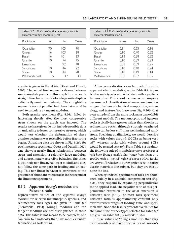
Representative values of the apparent Young’s
modulus for selected metamorphic, igneous, and
sedimentary rock types are given in Table 8.2
(Bieniawski, 1984). Young’s modulus and the
tangent modulus are not distinguished in these
data. This table is not meant to be complete: one
can turn to handbooks that have more extensive
tabulations (Clark, 1966).
A few generalizations can be made from the
apparent elastic moduli given in Table 8.2. A particular rock type is not associated with a particular modulus. This should come as no surprise
because rock classification schemes are based on
ranges of values of chemical composition, mineralogy, and texture. You have seen (Fig. 8.26b) that
even samples from the same rock mass can exhibit
different moduli. The metamorphic and igneous
rocks typically have greater values than the clastic
sedimentary rocks, although strongly weathered
granite can be less stiff than well-indurated sandstone. Speaking qualitatively, we would describe
rocks with values around 100 GPa as being very
stiff, whereas rocks with values around 1 GPa
would be termed very soft. From Table 8.2 we draw
the following rule of thumb: laboratory specimens of
rock have Young’s moduli that range from about 1 to
100 GPa with a “typical” value of about 50 GPa. Rocks
are very stiff relative to our experience with softer
elastic materials like rubber, but they are elastic
none-the-less.
When cylindrical specimens of rock are shortened axially in a uniaxial compression test (Fig.
8.25), they respond by expanding perpendicular
to the applied load. The negative ratio of this perpendicular extension to the axial extension is
Poisson’s ratio (8.10). For most rock specimens
Poisson’s ratio is approximately constant only
over restricted ranges of loading, time, and specimen size. None-the-less, representative values for
the same suite of rock types selected for Table 8.2
are given in Table 8.3 (Bieniawski, 1984).
Unlike values of Young’s modulus that vary
over two orders of magnitude, values of Poisson’s
8.5 LABORATORY AND ENGINEERING FIELD TESTS
321
Table 8.2. Rock mechanics laboratory tests for
apparent Young’s modulus (GPa).
Rock type
From
To
Mean
Quartzite
70
105
90
Gneiss
16
103
68
Basalt
16
101
63
Granite
10
74
45
Limestone
1
92
48
Sandstone
10
46
22
Shale
10
44
28
Pittsburgh coal
1.5
3.7
3.2
Table 8.3. Rock mechanics laboratory tests for
apparent Poisson’s ratio.
Rock type
From
To
Mean
Quartzite
0.11
0.25
0.16
Gneiss
0.10
0.40
0.22
Basalt
0.13
0.38
0.22
Granite
0.10
0.39
0.23
Limestone
0.08
0.39
0.25
Sandstone
0.10
0.40
0.24
Shale
0.10
0.19
0.14
Witbank coal
0.33
0.37
0.35
1967). The set of line segments drawn between
successive data points on this graph form a nearly
straight line. In contrast Colorado granite displays
a distinctly non-linear behavior. The straight-line
segments are not parallel, but these data could be
used to calculate a tangent modulus.
Both granite specimens (Fig. 8.26a) failed by
fracturing shortly after the most compressive
stress shown on the graph was imposed. The
results we have given do not include possible data
on unloading to lesser compressive stresses, which
would test whether the deformation of these
granite specimens was reversible before fracturing
began. Unloading data are shown in Fig. 8.26b for
two limestone specimens (Obert and Duvall, 1967).
One shows a nearly linear relationship between
stress and extension, a relatively large modulus,
and approximately reversible behavior. The other
is distinctly non-linear, has lesser moduli, and does
not follow the same path in loading and unloading. This non-linear behavior is attributed to the
presence of abundant microcracks in the second of
the limestone specimens.
8.5.2 Apparent Young’s modulus and
Poisson’s ratio
Representative values of the apparent Young’s
modulus for selected metamorphic, igneous, and
sedimentary rock types are given in Table 8.2
(Bieniawski, 1984). Young’s modulus and the
tangent modulus are not distinguished in these
data. This table is not meant to be complete: one
can turn to handbooks that have more extensive
tabulations (Clark, 1966).
A few generalizations can be made from the
apparent elastic moduli given in Table 8.2. A particular rock type is not associated with a particular modulus. This should come as no surprise
because rock classification schemes are based on
ranges of values of chemical composition, mineralogy, and texture. You have seen (Fig. 8.26b) that
even samples from the same rock mass can exhibit
different moduli. The metamorphic and igneous
rocks typically have greater values than the clastic
sedimentary rocks, although strongly weathered
granite can be less stiff than well-indurated sandstone. Speaking qualitatively, we would describe
rocks with values around 100 GPa as being very
stiff, whereas rocks with values around 1 GPa
would be termed very soft. From Table 8.2 we draw
the following rule of thumb: laboratory specimens of
rock have Young’s moduli that range from about 1 to
100 GPa with a “typical” value of about 50 GPa. Rocks
are very stiff relative to our experience with softer
elastic materials like rubber, but they are elastic
none-the-less.
When cylindrical specimens of rock are shortened axially in a uniaxial compression test (Fig.
8.25), they respond by expanding perpendicular
to the applied load. The negative ratio of this perpendicular extension to the axial extension is
Poisson’s ratio (8.10). For most rock specimens
Poisson’s ratio is approximately constant only
over restricted ranges of loading, time, and specimen size. None-the-less, representative values for
the same suite of rock types selected for Table 8.2
are given in Table 8.3 (Bieniawski, 1984).
Unlike values of Young’s modulus that vary
over two orders of magnitude, values of Poisson’s
8.5 LABORATORY AND ENGINEERING FIELD TESTS
321
Table 8.2. Rock mechanics laboratory tests for
apparent Young’s modulus (GPa).
Rock type
From
To
Mean
Quartzite
70
105
90
Gneiss
16
103
68
Basalt
16
101
63
Granite
10
74
45
Limestone
1
92
48
Sandstone
10
46
22
Shale
10
44
28
Pittsburgh coal
1.5
3.7
3.2
Table 8.3. Rock mechanics laboratory tests for
apparent Poisson’s ratio.
Rock type
From
To
Mean
Quartzite
0.11
0.25
0.16
Gneiss
0.10
0.40
0.22
Basalt
0.13
0.38
0.22
Granite
0.10
0.39
0.23
Limestone
0.08
0.39
0.25
Sandstone
0.10
0.40
0.24
Shale
0.10
0.19
0.14
Witbank coal
0.33
0.37
0.35