

(8.76)
(8.77)
To solve a particular problem the stress components must satisfy the specified traction boundary
conditions following Cauchy’s Formula.
Hooke’s Law is defined by noting that one may
rotate the Cartesian coordinates (x, y) about the zaxis to coincide with the polar coordinates (r, ).
Then, the strain–stress relationships in polar
coordinates are written by exchanging each
Cartesian subscript in (8.48)–(8.50) with its polar
counterpart:
(8.78)
(8.79)
(8.80)
The kinematic equations in polar coordinates are
(Malvern, 1969):
(8.81)
(8.82)
(8.83)
The three strain components are used to determine two displacement components, so these
strains must satisfy a compatibility condition
which is written in terms of the Airy stress function, giving the biharmonic equation in polar
coordinates (Malvern, 1969):
(8.84)
Solutions to this equation for stress states that
satisfy particular boundary conditions are
reviewed in textbooks on elasticity theory
(Timoshenko and Goodier, 1970; Barber, 1992).
Ѩ 2
Ѩr 2 ϩ
1
r
Ѩ
Ѩr
ϩ
1
r 2
Ѩ 2
Ѩ 2
Ѩ 2 ⌽
Ѩr 2 ϩ
1
r
Ѩ⌽
Ѩr
ϩ
1
r 2
Ѩ 2 ⌽
Ѩ 2 ϭ 0
r ϭ
1
2r
Ѩu r
Ѩ
ϩ r
Ѩu
Ѩr
Ϫ u
ϭ
1
r
u r ϩ
Ѩu
Ѩ
rr ϭ
Ѩu r
Ѩr
r ϭ
1 ϩ
E
r
ϭ
1
E
[ (1 Ϫ 2 ) Ϫ rr (1 ϩ )]
rr ϭ
1
E
[ rr (1 Ϫ 2 ) Ϫ (1 ϩ )]
ϭ
Ѩ 2 ⌽
Ѩr 2 ϩ g*r sin
r ϭ Ϫ
Ѩ
Ѩr
1
r
Ѩ⌽
Ѩ
In 1899, J. H. Michell derived a generalized
Airy stress function in polar coordinates, from
which many particular solutions can be extracted
(Michell, 1899; Timoshenko and Goodier, 1970):
314
ELASTIC DEFORMATION
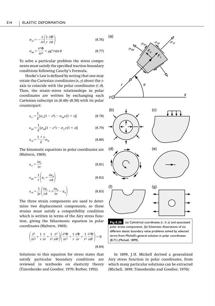
Fig 8.20 (a) Cylindrical coordinates (r, , z) and associated
polar stress components. (b) Schematic illustrations of six
different elastic boundary value problems solved by selected
terms from Michell’s general solution in polar coordinates
(8.71) (Michell, 1899).
s ur
x
r
u
s uu
s rr
s ru
(a)
(b)
(d)
(c)
(e)
(f)
(g)
F r
F u
z
(8.77)
To solve a particular problem the stress components must satisfy the specified traction boundary
conditions following Cauchy’s Formula.
Hooke’s Law is defined by noting that one may
rotate the Cartesian coordinates (x, y) about the zaxis to coincide with the polar coordinates (r, ).
Then, the strain–stress relationships in polar
coordinates are written by exchanging each
Cartesian subscript in (8.48)–(8.50) with its polar
counterpart:
(8.78)
(8.79)
(8.80)
The kinematic equations in polar coordinates are
(Malvern, 1969):
(8.81)
(8.82)
(8.83)
The three strain components are used to determine two displacement components, so these
strains must satisfy a compatibility condition
which is written in terms of the Airy stress function, giving the biharmonic equation in polar
coordinates (Malvern, 1969):
(8.84)
Solutions to this equation for stress states that
satisfy particular boundary conditions are
reviewed in textbooks on elasticity theory
(Timoshenko and Goodier, 1970; Barber, 1992).
Ѩ 2
Ѩr 2 ϩ
1
r
Ѩ
Ѩr
ϩ
1
r 2
Ѩ 2
Ѩ 2
Ѩ 2 ⌽
Ѩr 2 ϩ
1
r
Ѩ⌽
Ѩr
ϩ
1
r 2
Ѩ 2 ⌽
Ѩ 2 ϭ 0
r ϭ
1
2r
Ѩu r
Ѩ
ϩ r
Ѩu
Ѩr
Ϫ u
ϭ
1
r
u r ϩ
Ѩu
Ѩ
rr ϭ
Ѩu r
Ѩr
r ϭ
1 ϩ
E
r
ϭ
1
E
[ (1 Ϫ 2 ) Ϫ rr (1 ϩ )]
rr ϭ
1
E
[ rr (1 Ϫ 2 ) Ϫ (1 ϩ )]
ϭ
Ѩ 2 ⌽
Ѩr 2 ϩ g*r sin
r ϭ Ϫ
Ѩ
Ѩr
1
r
Ѩ⌽
Ѩ
In 1899, J. H. Michell derived a generalized
Airy stress function in polar coordinates, from
which many particular solutions can be extracted
(Michell, 1899; Timoshenko and Goodier, 1970):
314
ELASTIC DEFORMATION
Fig 8.20 (a) Cylindrical coordinates (r, , z) and associated
polar stress components. (b) Schematic illustrations of six
different elastic boundary value problems solved by selected
terms from Michell’s general solution in polar coordinates
(8.71) (Michell, 1899).
s ur
x
r
u
s uu
s rr
s ru
(a)
(b)
(d)
(c)
(e)
(f)
(g)
F r
F u
z