

therefore would be a physically inappropriate
application of this solution.
If the region of interest is entirely below the
traction-free surface, (8.55) can be modified to
account for a translation of the origin to a depth,
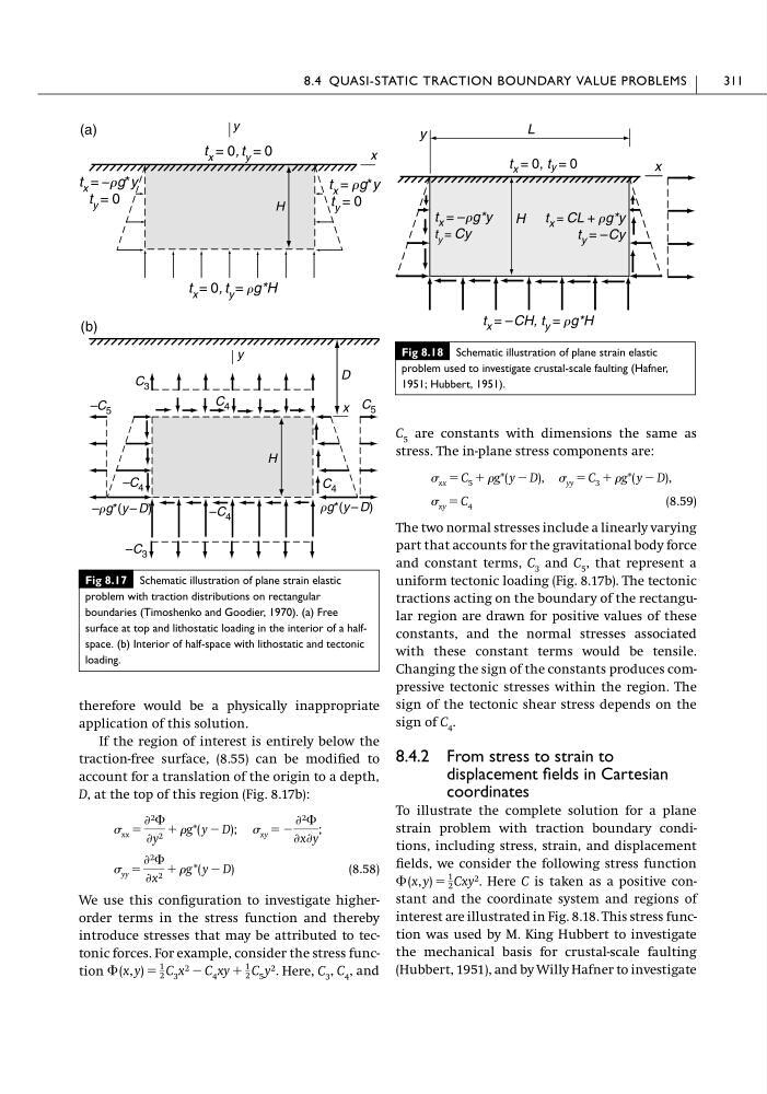
D, at the top of this region (Fig. 8.17b):
(8.58)
We use this configuration to investigate higherorder terms in the stress function and thereby
introduce stresses that may be attributed to tectonic forces. For example, consider the stress function
Here, C 3 , C 4 , and
⌽ (x, y) ϭ
1
2 C 3 x 2 Ϫ C 4 xy ϩ
1
2 C 5 y 2 .
yy ϭ
Ѩ 2 ⌽
Ѩx 2 ϩ g *( y Ϫ D)
xx ϭ
Ѩ 2 ⌽
Ѩy 2 ϩ g*( y Ϫ D); xy ϭ Ϫ
Ѩ 2 ⌽
ѨxѨy
;
C 5 are constants with dimensions the same as
stress. The in-plane stress components are:
(8.59)
The two normal stresses include a linearly varying
part that accounts for the gravitational body force
and constant terms, C 3 and C 5 , that represent a
uniform tectonic loading (Fig. 8.17b). The tectonic
tractions acting on the boundary of the rectangular region are drawn for positive values of these
constants, and the normal stresses associated
with these constant terms would be tensile.
Changing the sign of the constants produces compressive tectonic stresses within the region. The
sign of the tectonic shear stress depends on the
sign of C 4 .
8.4.2 From stress to strain to
displacement fields in Cartesian
coordinates
To illustrate the complete solution for a plane
strain problem with traction boundary conditions, including stress, strain, and displacement
fields, we consider the following stress function
Here C is taken as a positive constant and the coordinate system and regions of
interest are illustrated in Fig. 8.18. This stress function was used by M. King Hubbert to investigate
the mechanical basis for crustal-scale faulting
(Hubbert, 1951), and by Willy Hafner to investigate
⌽ (x, y) ϭ
1
2 Cxy 2 .
xy ϭ C 4
xx ϭ C 5 ϩ g*( y Ϫ D), yy ϭ C 3 ϩ g*( y Ϫ D),
8.4 QUASI-STATIC TRACTION BOUNDARY VALUE PROBLEMS
311
Fig 8.17 Schematic illustration of plane strain elastic
problem with traction distributions on rectangular
boundaries (Timoshenko and Goodier, 1970). (a) Free
surface at top and lithostatic loading in the interior of a halfspace. (b) Interior of half-space with lithostatic and tectonic
loading.
(a)
x
y
H
(b)
x
y
H
t x = –rg*y
t y = 0
t x = 0, t y = rg*H
t x = 0, t y = 0
C 3
D
t x = rg*y
t y = 0
C 4
–C 3
–C 4
–C 4
C 4
–C 5
C 5
–rg*(y – D)
rg*(y – D)
Fig 8.18 Schematic illustration of plane strain elastic
problem used to investigate crustal-scale faulting (Hafner,
1951; Hubbert, 1951).
x
y
H
L
t x = CL + rg*y
t y = –Cy
t x = –CH, t y = rg*H
t x = –rg*y
t y = Cy
t x = 0, t y = 0
application of this solution.
If the region of interest is entirely below the
traction-free surface, (8.55) can be modified to
account for a translation of the origin to a depth,
D, at the top of this region (Fig. 8.17b):
(8.58)
We use this configuration to investigate higherorder terms in the stress function and thereby
introduce stresses that may be attributed to tectonic forces. For example, consider the stress function
Here, C 3 , C 4 , and
⌽ (x, y) ϭ
1
2 C 3 x 2 Ϫ C 4 xy ϩ
1
2 C 5 y 2 .
yy ϭ
Ѩ 2 ⌽
Ѩx 2 ϩ g *( y Ϫ D)
xx ϭ
Ѩ 2 ⌽
Ѩy 2 ϩ g*( y Ϫ D); xy ϭ Ϫ
Ѩ 2 ⌽
ѨxѨy
;
C 5 are constants with dimensions the same as
stress. The in-plane stress components are:
(8.59)
The two normal stresses include a linearly varying
part that accounts for the gravitational body force
and constant terms, C 3 and C 5 , that represent a
uniform tectonic loading (Fig. 8.17b). The tectonic
tractions acting on the boundary of the rectangular region are drawn for positive values of these
constants, and the normal stresses associated
with these constant terms would be tensile.
Changing the sign of the constants produces compressive tectonic stresses within the region. The
sign of the tectonic shear stress depends on the
sign of C 4 .
8.4.2 From stress to strain to
displacement fields in Cartesian
coordinates
To illustrate the complete solution for a plane
strain problem with traction boundary conditions, including stress, strain, and displacement
fields, we consider the following stress function
Here C is taken as a positive constant and the coordinate system and regions of
interest are illustrated in Fig. 8.18. This stress function was used by M. King Hubbert to investigate
the mechanical basis for crustal-scale faulting
(Hubbert, 1951), and by Willy Hafner to investigate
⌽ (x, y) ϭ
1
2 Cxy 2 .
xy ϭ C 4
xx ϭ C 5 ϩ g*( y Ϫ D), yy ϭ C 3 ϩ g*( y Ϫ D),
8.4 QUASI-STATIC TRACTION BOUNDARY VALUE PROBLEMS
311
Fig 8.17 Schematic illustration of plane strain elastic
problem with traction distributions on rectangular
boundaries (Timoshenko and Goodier, 1970). (a) Free
surface at top and lithostatic loading in the interior of a halfspace. (b) Interior of half-space with lithostatic and tectonic
loading.
(a)
x
y
H
(b)
x
y
H
t x = –rg*y
t y = 0
t x = 0, t y = rg*H
t x = 0, t y = 0
C 3
D
t x = rg*y
t y = 0
C 4
–C 3
–C 4
–C 4
C 4
–C 5
C 5
–rg*(y – D)
rg*(y – D)
Fig 8.18 Schematic illustration of plane strain elastic
problem used to investigate crustal-scale faulting (Hafner,
1951; Hubbert, 1951).
x
y
H
L
t x = CL + rg*y
t y = –Cy
t x = –CH, t y = rg*H
t x = –rg*y
t y = Cy
t x = 0, t y = 0