

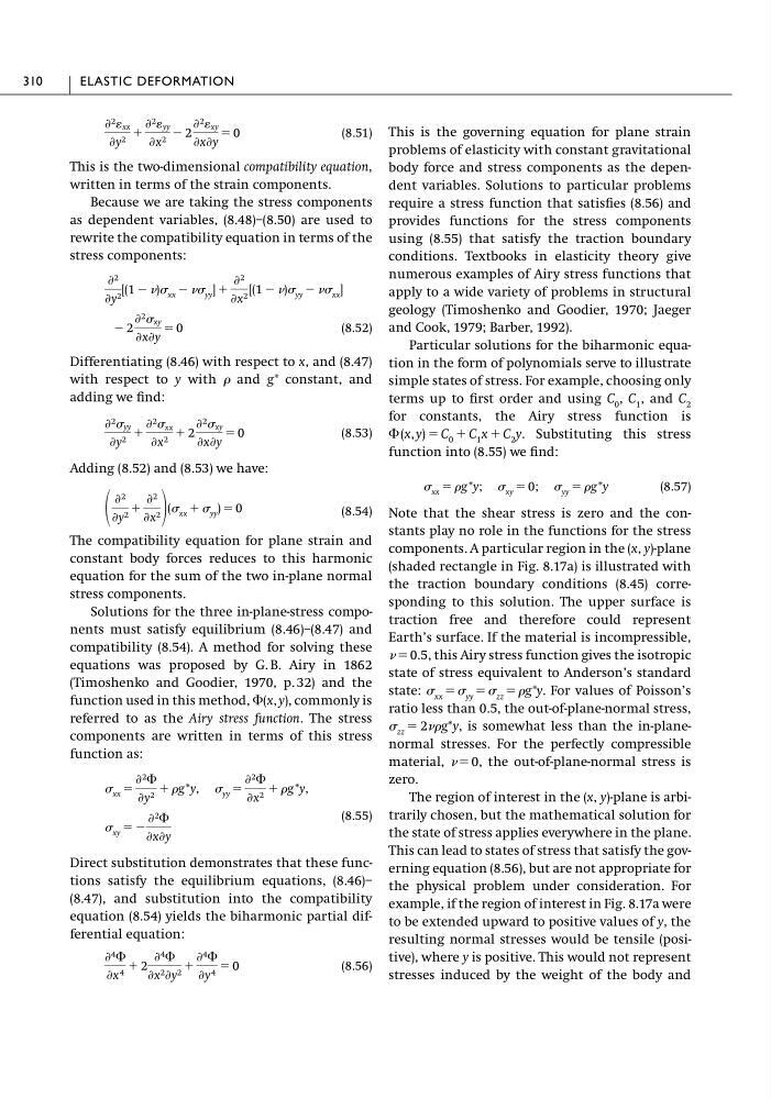
(8.51)
This is the two-dimensional compatibility equation,
written in terms of the strain components.
Because we are taking the stress components
as dependent variables, (8.48)–(8.50) are used to
rewrite the compatibility equation in terms of the
stress components:
(8.52)
Differentiating (8.46) with respect to x, and (8.47)
with respect to y with and g* constant, and
adding we find:
(8.53)
Adding (8.52) and (8.53) we have:
(8.54)
The compatibility equation for plane strain and
constant body forces reduces to this harmonic
equation for the sum of the two in-plane normal
stress components.
Solutions for the three in-plane-stress components must satisfy equilibrium (8.46)–(8.47) and
compatibility (8.54). A method for solving these
equations was proposed by G. B. Airy in 1862
(Timoshenko and Goodier, 1970, p. 32) and the
function used in this method, ⌽(x, y), commonly is
referred to as the Airy stress function. The stress
components are written in terms of this stress
function as:
(8.55)
Direct substitution demonstrates that these functions satisfy the equilibrium equations, (8.46)–
(8.47), and substitution into the compatibility
equation (8.54) yields the biharmonic partial differential equation:
(8.56)
Ѩ 4 ⌽
Ѩx 4 ϩ 2
Ѩ 4 ⌽
Ѩx 2 Ѩy 2 ϩ
Ѩ 4 ⌽
Ѩy 4 ϭ 0
xy ϭ Ϫ
Ѩ 2 ⌽
ѨxѨy
xx ϭ
Ѩ 2 ⌽
Ѩy 2 ϩ g *y, yy ϭ
Ѩ 2 ⌽
Ѩx 2 ϩ g *y,
Ѩ 2
Ѩy 2 ϩ
Ѩ 2
Ѩx 2 ( xx ϩ yy ) ϭ 0
Ѩ 2 yy
Ѩy 2 ϩ
Ѩ 2 xx
Ѩx 2 ϩ 2
Ѩ 2 xy
ѨxѨy
ϭ 0
Ϫ 2
Ѩ 2 xy
ѨxѨy
ϭ 0
ϩ
Ѩ 2
Ѩx 2 [(1 Ϫ ) yy Ϫ xx ]
Ѩ 2
Ѩy 2 [(1 Ϫ ) xx Ϫ yy ]
Ѩ 2 xx
Ѩy 2 ϩ
Ѩ 2 yy
Ѩx 2 Ϫ 2
Ѩ 2 xy
ѨxѨy
ϭ 0
This is the governing equation for plane strain
problems of elasticity with constant gravitational
body force and stress components as the dependent variables. Solutions to particular problems
require a stress function that satisfies (8.56) and
provides functions for the stress components
using (8.55) that satisfy the traction boundary
conditions. Textbooks in elasticity theory give
numerous examples of Airy stress functions that
apply to a wide variety of problems in structural
geology (Timoshenko and Goodier, 1970; Jaeger
and Cook, 1979; Barber, 1992).
Particular solutions for the biharmonic equation in the form of polynomials serve to illustrate
simple states of stress. For example, choosing only
terms up to first order and using C 0 , C 1 , and C 2
for constants, the Airy stress function is
Substituting this stress
function into (8.55) we find:
(8.57)
Note that the shear stress is zero and the constants play no role in the functions for the stress
components. A particular region in the (x, y)-plane
(shaded rectangle in Fig. 8.17a) is illustrated with
the traction boundary conditions (8.45) corresponding to this solution. The upper surface is
traction free and therefore could represent
Earth’s surface. If the material is incompressible,
ϭ 0.5, this Airy stress function gives the isotropic
state of stress equivalent to Anderson’s standard
state: xx ϭ yy ϭ zz ϭ g*y. For values of Poisson’s
ratio less than 0.5, the out-of-plane-normal stress,
is somewhat less than the in-planenormal stresses. For the perfectly compressible
material, ϭ 0, the out-of-plane-normal stress is
zero.
The region of interest in the (x, y)-plane is arbitrarily chosen, but the mathematical solution for
the state of stress applies everywhere in the plane.
This can lead to states of stress that satisfy the governing equation (8.56), but are not appropriate for
the physical problem under consideration. For
example, if the region of interest in Fig. 8.17a were
to be extended upward to positive values of y, the
resulting normal stresses would be tensile (positive), where y is positive. This would not represent
stresses induced by the weight of the body and
zz ϭ 2g*y,
xx ϭ g *y; xy ϭ 0; yy ϭ g *y
⌽ (x, y) ϭ C 0 ϩ C 1 x ϩ C 2 y.
310
ELASTIC DEFORMATION
This is the two-dimensional compatibility equation,
written in terms of the strain components.
Because we are taking the stress components
as dependent variables, (8.48)–(8.50) are used to
rewrite the compatibility equation in terms of the
stress components:
(8.52)
Differentiating (8.46) with respect to x, and (8.47)
with respect to y with and g* constant, and
adding we find:
(8.53)
Adding (8.52) and (8.53) we have:
(8.54)
The compatibility equation for plane strain and
constant body forces reduces to this harmonic
equation for the sum of the two in-plane normal
stress components.
Solutions for the three in-plane-stress components must satisfy equilibrium (8.46)–(8.47) and
compatibility (8.54). A method for solving these
equations was proposed by G. B. Airy in 1862
(Timoshenko and Goodier, 1970, p. 32) and the
function used in this method, ⌽(x, y), commonly is
referred to as the Airy stress function. The stress
components are written in terms of this stress
function as:
(8.55)
Direct substitution demonstrates that these functions satisfy the equilibrium equations, (8.46)–
(8.47), and substitution into the compatibility
equation (8.54) yields the biharmonic partial differential equation:
(8.56)
Ѩ 4 ⌽
Ѩx 4 ϩ 2
Ѩ 4 ⌽
Ѩx 2 Ѩy 2 ϩ
Ѩ 4 ⌽
Ѩy 4 ϭ 0
xy ϭ Ϫ
Ѩ 2 ⌽
ѨxѨy
xx ϭ
Ѩ 2 ⌽
Ѩy 2 ϩ g *y, yy ϭ
Ѩ 2 ⌽
Ѩx 2 ϩ g *y,
Ѩ 2
Ѩy 2 ϩ
Ѩ 2
Ѩx 2 ( xx ϩ yy ) ϭ 0
Ѩ 2 yy
Ѩy 2 ϩ
Ѩ 2 xx
Ѩx 2 ϩ 2
Ѩ 2 xy
ѨxѨy
ϭ 0
Ϫ 2
Ѩ 2 xy
ѨxѨy
ϭ 0
ϩ
Ѩ 2
Ѩx 2 [(1 Ϫ ) yy Ϫ xx ]
Ѩ 2
Ѩy 2 [(1 Ϫ ) xx Ϫ yy ]
Ѩ 2 xx
Ѩy 2 ϩ
Ѩ 2 yy
Ѩx 2 Ϫ 2
Ѩ 2 xy
ѨxѨy
ϭ 0
This is the governing equation for plane strain
problems of elasticity with constant gravitational
body force and stress components as the dependent variables. Solutions to particular problems
require a stress function that satisfies (8.56) and
provides functions for the stress components
using (8.55) that satisfy the traction boundary
conditions. Textbooks in elasticity theory give
numerous examples of Airy stress functions that
apply to a wide variety of problems in structural
geology (Timoshenko and Goodier, 1970; Jaeger
and Cook, 1979; Barber, 1992).
Particular solutions for the biharmonic equation in the form of polynomials serve to illustrate
simple states of stress. For example, choosing only
terms up to first order and using C 0 , C 1 , and C 2
for constants, the Airy stress function is
Substituting this stress
function into (8.55) we find:
(8.57)
Note that the shear stress is zero and the constants play no role in the functions for the stress
components. A particular region in the (x, y)-plane
(shaded rectangle in Fig. 8.17a) is illustrated with
the traction boundary conditions (8.45) corresponding to this solution. The upper surface is
traction free and therefore could represent
Earth’s surface. If the material is incompressible,
ϭ 0.5, this Airy stress function gives the isotropic
state of stress equivalent to Anderson’s standard
state: xx ϭ yy ϭ zz ϭ g*y. For values of Poisson’s
ratio less than 0.5, the out-of-plane-normal stress,
is somewhat less than the in-planenormal stresses. For the perfectly compressible
material, ϭ 0, the out-of-plane-normal stress is
zero.
The region of interest in the (x, y)-plane is arbitrarily chosen, but the mathematical solution for
the state of stress applies everywhere in the plane.
This can lead to states of stress that satisfy the governing equation (8.56), but are not appropriate for
the physical problem under consideration. For
example, if the region of interest in Fig. 8.17a were
to be extended upward to positive values of y, the
resulting normal stresses would be tensile (positive), where y is positive. This would not represent
stresses induced by the weight of the body and
zz ϭ 2g*y,
xx ϭ g *y; xy ϭ 0; yy ϭ g *y
⌽ (x, y) ϭ C 0 ϩ C 1 x ϩ C 2 y.
310
ELASTIC DEFORMATION