

dependent variables are the three in-plane stress
components which only are functions of x and y:
(8.44)
The out-of-plane-normal stress is given by (8.35),
and the out-of-plane shear stresses are zero.
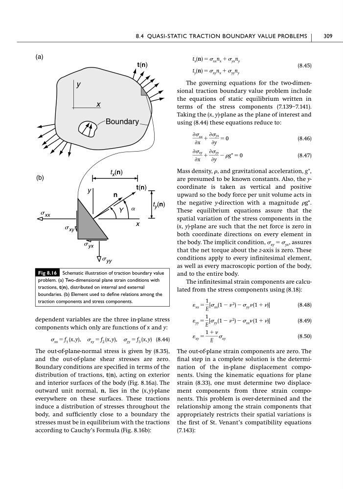
Boundary conditions are specified in terms of the
distribution of tractions, t(n), acting on exterior
and interior surfaces of the body (Fig. 8.16a). The
outward unit normal, n, lies in the (x, y)-plane
everywhere on these surfaces. These tractions
induce a distribution of stresses throughout the
body, and sufficiently close to a boundary the
stresses must be in equilibrium with the tractions
according to Cauchy’s Formula (Fig. 8.16b):
xx ϭ f 1 (x, y), xy ϭ f 2 (x, y), yy ϭ f 3 (x, y)
(8.45)
The governing equations for the two-dimensional traction boundary value problem include
the equations of static equilibrium written in
terms of the stress components (7.139–7.141).
Taking the (x, y)-plane as the plane of interest and
using (8.44) these equations reduce to:
(8.46)
(8.47)
Mass density, , and gravitational acceleration, g*,
are presumed to be known constants. Also, the ycoordinate is taken as vertical and positive
upward so the body force per unit volume acts in
the negative y-direction with a magnitude g*.
These equilibrium equations assure that the
spatial variation of the stress components in the
(x, y)-plane are such that the net force is zero in
both coordinate directions on every element in
the body. The implicit condition,
assures
that the net torque about the z-axis is zero. These
conditions apply to every infinitesimal element,
as well as every macroscopic portion of the body,
and to the entire body.
The infinitesimal strain components are calculated from the stress components using (8.18):
(8.48)
(8.49)
(8.50)
The out-of-plane strain components are zero. The
final step in a complete solution is the determination of the in-plane displacement components. Using the kinematic equations for plane
strain (8.33), one must determine two displacement components from three strain components. This problem is over-determined and the
relationship among the strain components that
appropriately restricts their spatial variations is
the first of St. Venant’s compatibility equations
(7.143):
xy ϭ
1 ϩ
E
xy
yy ϭ
1
E
[ yy (1 Ϫ 2 ) Ϫ xx (1 ϩ )]
xx ϭ
1
E
[ xx (1 Ϫ 2 ) Ϫ yy (1 ϩ )]
xy ϭ yx ,
Ѩ xy
Ѩx
ϩ
Ѩ yy
Ѩy
Ϫ g* ϭ 0
Ѩ xx
Ѩx
ϩ
Ѩ yx
Ѩy
ϭ 0
t y (n) ϭ xy n x ϩ yy n y
t x (n) ϭ xx n x ϩ yx n y
8.4 QUASI-STATIC TRACTION BOUNDARY VALUE PROBLEMS
309
Fig 8.16 Schematic illustration of traction boundary value
problem. (a) Two-dimensional plane strain conditions with
tractions, t(n), distributed on internal and external
boundaries. (b) Element used to define relations among the
traction components and stress components.
(a)
Boundary
s xx
s xy
s yx
s yy
x
y
n
(b)
Y a
x
y
t x (n)
t y (n)
t(n)
t(n)
components which only are functions of x and y:
(8.44)
The out-of-plane-normal stress is given by (8.35),
and the out-of-plane shear stresses are zero.
Boundary conditions are specified in terms of the
distribution of tractions, t(n), acting on exterior
and interior surfaces of the body (Fig. 8.16a). The
outward unit normal, n, lies in the (x, y)-plane
everywhere on these surfaces. These tractions
induce a distribution of stresses throughout the
body, and sufficiently close to a boundary the
stresses must be in equilibrium with the tractions
according to Cauchy’s Formula (Fig. 8.16b):
xx ϭ f 1 (x, y), xy ϭ f 2 (x, y), yy ϭ f 3 (x, y)
(8.45)
The governing equations for the two-dimensional traction boundary value problem include
the equations of static equilibrium written in
terms of the stress components (7.139–7.141).
Taking the (x, y)-plane as the plane of interest and
using (8.44) these equations reduce to:
(8.46)
(8.47)
Mass density, , and gravitational acceleration, g*,
are presumed to be known constants. Also, the ycoordinate is taken as vertical and positive
upward so the body force per unit volume acts in
the negative y-direction with a magnitude g*.
These equilibrium equations assure that the
spatial variation of the stress components in the
(x, y)-plane are such that the net force is zero in
both coordinate directions on every element in
the body. The implicit condition,
assures
that the net torque about the z-axis is zero. These
conditions apply to every infinitesimal element,
as well as every macroscopic portion of the body,
and to the entire body.
The infinitesimal strain components are calculated from the stress components using (8.18):
(8.48)
(8.49)
(8.50)
The out-of-plane strain components are zero. The
final step in a complete solution is the determination of the in-plane displacement components. Using the kinematic equations for plane
strain (8.33), one must determine two displacement components from three strain components. This problem is over-determined and the
relationship among the strain components that
appropriately restricts their spatial variations is
the first of St. Venant’s compatibility equations
(7.143):
xy ϭ
1 ϩ
E
xy
yy ϭ
1
E
[ yy (1 Ϫ 2 ) Ϫ xx (1 ϩ )]
xx ϭ
1
E
[ xx (1 Ϫ 2 ) Ϫ yy (1 ϩ )]
xy ϭ yx ,
Ѩ xy
Ѩx
ϩ
Ѩ yy
Ѩy
Ϫ g* ϭ 0
Ѩ xx
Ѩx
ϩ
Ѩ yx
Ѩy
ϭ 0
t y (n) ϭ xy n x ϩ yy n y
t x (n) ϭ xx n x ϩ yx n y
8.4 QUASI-STATIC TRACTION BOUNDARY VALUE PROBLEMS
309
Fig 8.16 Schematic illustration of traction boundary value
problem. (a) Two-dimensional plane strain conditions with
tractions, t(n), distributed on internal and external
boundaries. (b) Element used to define relations among the
traction components and stress components.
(a)
Boundary
s xx
s xy
s yx
s yy
x
y
n
(b)
Y a
x
y
t x (n)
t y (n)
t(n)
t(n)