

to calculate the range, or distance, from the satellite to each reflective site on the surface. If the
same region is imaged at two different times, and
if the reflectivity of the surface has not changed
significantly, the difference between the two
images can be used to calculate the component of
the surface displacement directed along the line
between the satellite and the ground surface for
each pixel. Because the satellite will not be in precisely the same position for the two images the
effects of the topography must be removed. The
resulting image is called an interferogram. Note
that the data contained on the interferogram are
not the displacement vector at each pixel, but one
component of that vector.
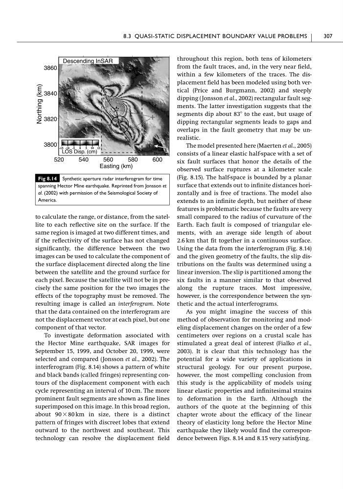
To investigate deformation associated with
the Hector Mine earthquake, SAR images for
September 15, 1999, and October 20, 1999, were
selected and compared (Jonsson et al., 2002). The
interferogram (Fig. 8.14) shows a pattern of white
and black bands (called fringes) representing contours of the displacement component with each
cycle representing an interval of 10 cm. The more
prominent fault segments are shown as fine lines
superimposed on this image. In this broad region,
about 90 ϫ 80 km in size, there is a distinct
pattern of fringes with discreet lobes that extend
outward to the northwest and southeast. This
technology can resolve the displacement field
throughout this region, both tens of kilometers
from the fault traces, and, in the very near field,
within a few kilometers of the traces. The displacement field has been modeled using both vertical (Price and Burgmann, 2002) and steeply
dipping ( Jonsson et al., 2002) rectangular fault segments. The latter investigation suggests that the
segments dip about 83Њ to the east, but usage of
dipping rectangular segments leads to gaps and
overlaps in the fault geometry that may be unrealistic.
The model presented here (Maerten et al., 2005)
consists of a linear elastic half-space with a set of
six fault surfaces that honor the details of the
observed surface ruptures at a kilometer scale
(Fig. 8.15). The half-space is bounded by a planar
surface that extends out to infinite distances horizontally and is free of tractions. The model also
extends to an infinite depth, but neither of these
features is problematic because the faults are very
small compared to the radius of curvature of the
Earth. Each fault is composed of triangular elements, with an average side length of about
2.6 km that fit together in a continuous surface.
Using the data from the interferogram (Fig. 8.14)
and the given geometry of the faults, the slip distributions on the faults was determined using a
linear inversion. The slip is partitioned among the
six faults in a manner similar to that observed
along the rupture traces. Most impressive,
however, is the correspondence between the synthetic and the actual interferograms.
As you might imagine the success of this
method of observation for monitoring and modeling displacement changes on the order of a few
centimeters over regions on a crustal scale has
stimulated a great deal of interest (Fialko et al.,
2003). It is clear that this technology has the
potential for a wide variety of applications in
structural geology. For our present purpose,
however, the most compelling conclusion from
this study is the applicability of models using
linear elastic properties and infinitesimal strains
to deformation in the Earth. Although the
authors of the quote at the beginning of this
chapter wrote about the efficacy of the linear
theory of elasticity long before the Hector Mine
earthquake they likely would find the correspondence between Figs. 8.14 and 8.15 very satisfying.
8.3 QUASI-STATIC DISPLACEMENT BOUNDARY VALUE PROBLEMS
307
Fig 8.14 Synthetic aperture radar interferogram for time
spanning Hector Mine earthquake. Reprinted from Jonsson et
al. (2002) with permission of the Seismological Society of
America.
same region is imaged at two different times, and
if the reflectivity of the surface has not changed
significantly, the difference between the two
images can be used to calculate the component of
the surface displacement directed along the line
between the satellite and the ground surface for
each pixel. Because the satellite will not be in precisely the same position for the two images the
effects of the topography must be removed. The
resulting image is called an interferogram. Note
that the data contained on the interferogram are
not the displacement vector at each pixel, but one
component of that vector.
To investigate deformation associated with
the Hector Mine earthquake, SAR images for
September 15, 1999, and October 20, 1999, were
selected and compared (Jonsson et al., 2002). The
interferogram (Fig. 8.14) shows a pattern of white
and black bands (called fringes) representing contours of the displacement component with each
cycle representing an interval of 10 cm. The more
prominent fault segments are shown as fine lines
superimposed on this image. In this broad region,
about 90 ϫ 80 km in size, there is a distinct
pattern of fringes with discreet lobes that extend
outward to the northwest and southeast. This
technology can resolve the displacement field
throughout this region, both tens of kilometers
from the fault traces, and, in the very near field,
within a few kilometers of the traces. The displacement field has been modeled using both vertical (Price and Burgmann, 2002) and steeply
dipping ( Jonsson et al., 2002) rectangular fault segments. The latter investigation suggests that the
segments dip about 83Њ to the east, but usage of
dipping rectangular segments leads to gaps and
overlaps in the fault geometry that may be unrealistic.
The model presented here (Maerten et al., 2005)
consists of a linear elastic half-space with a set of
six fault surfaces that honor the details of the
observed surface ruptures at a kilometer scale
(Fig. 8.15). The half-space is bounded by a planar
surface that extends out to infinite distances horizontally and is free of tractions. The model also
extends to an infinite depth, but neither of these
features is problematic because the faults are very
small compared to the radius of curvature of the
Earth. Each fault is composed of triangular elements, with an average side length of about
2.6 km that fit together in a continuous surface.
Using the data from the interferogram (Fig. 8.14)
and the given geometry of the faults, the slip distributions on the faults was determined using a
linear inversion. The slip is partitioned among the
six faults in a manner similar to that observed
along the rupture traces. Most impressive,
however, is the correspondence between the synthetic and the actual interferograms.
As you might imagine the success of this
method of observation for monitoring and modeling displacement changes on the order of a few
centimeters over regions on a crustal scale has
stimulated a great deal of interest (Fialko et al.,
2003). It is clear that this technology has the
potential for a wide variety of applications in
structural geology. For our present purpose,
however, the most compelling conclusion from
this study is the applicability of models using
linear elastic properties and infinitesimal strains
to deformation in the Earth. Although the
authors of the quote at the beginning of this
chapter wrote about the efficacy of the linear
theory of elasticity long before the Hector Mine
earthquake they likely would find the correspondence between Figs. 8.14 and 8.15 very satisfying.
8.3 QUASI-STATIC DISPLACEMENT BOUNDARY VALUE PROBLEMS
307
Fig 8.14 Synthetic aperture radar interferogram for time
spanning Hector Mine earthquake. Reprinted from Jonsson et
al. (2002) with permission of the Seismological Society of
America.