

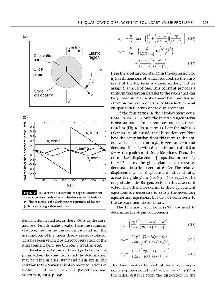
deformation would occur there. Outside the core,
and over length scales greater than the radius of
the core, the continuum concept is valid and the
assumptions of the linear theory are not violated.
This has been verified by direct observation of the
displacement field (see Chapter 8 frontispiece).
The elastic solution for the edge dislocation is
premised on the conditions that the deformation
may be taken as quasi-static and plain strain. The
solution to the Navier’s displacement equations of
motion, (8.31) and (8.32), is (Weertman and
Weertman, 1964, p. 36):
(8.36)
(8.37)
Here the arbitrary constant C in the expression for
u y has dimensions of length squared, so the argument of the log term is dimensionless, and we
assign C a value of one. This constant provides a
uniform translation parallel to the y-axis that can
be ignored in the displacement field and has no
effect on the strain or stress fields which depend
on spatial derivatives of the displacements.
Of the four terms in the displacement equations, (8.36)–(8.37), only the inverse tangent term
is discontinuous for a circuit around the dislocation line (Fig. 8.10b, u x term 1). Here the radius is
taken as r ϭ 10b, outside the dislocation core. Note
how the contribution from this term to the normalized displacement, u x /b, is zero at ϭ 0 and
decreases linearly with to a minimum of Ϫ0.5 at
ϭ , the position of the glide plane. Then, the
normalized displacement jumps discontinuously
to ϩ0.5 across the glide plane and thereafter
decreases linearly to zero at ϭ 2. The relative
displacement, or displacement discontinuity,
across the glide plane (x Յ 0, y ϭ 0) is equal to the
magnitude of the Burgers vector, in this case a unit
value. The other three terms in the displacement
equations are necessary to satisfy the governing
equilibrium equations, but do not contribute to
the displacement discontinuity.
The kinematic equations (8.33) are used to
determine the strain components:
(8.38)
(8.39)
(8.40)
The denominators for each of the strain components is proportional to r
4 where r ϭ (x
2 ϩ y
2 )
1/2 is
the radial distance from the dislocation in the
xy ϭ Ϫ
bx
2 ΄
2(G ϩ )(x 2 Ϫ y 2 )
(2G ϩ )(x 2 ϩ y 2 ) 2΅
yy ϭ Ϫ
by
2 ΄
(G ϩ 2)x 2 Ϫ Gy 2
(2G ϩ )(x 2 ϩ y 2 ) 2΅
xx ϭ
by
2 ΄
(3G ϩ 2)x 2 ϩ Gy 2
(2G ϩ )(x 2 ϩ y 2 ) 2 ΅
ϩ
G ϩ
2G ϩ
y 2
x 2 ϩ y 2 ΅
u y ϭ Ϫ
b
2
΄Ϫ
G
2(2G ϩ )
ln
x 2 ϩ y 2
C
u x ϭ Ϫ
b
2 ΄ tan Ϫ1
y
x ϩ
G ϩ
2G ϩ
xy
x 2 ϩ y 2 ΅
8.3 QUASI-STATIC DISPLACEMENT BOUNDARY VALUE PROBLEMS
303
Fig 8.10 (a) Schematic illustration of edge dislocation and
dislocation core inside of which the deformation is inelastic.
(b) Plot of terms in the displacement equations, (8.36) and
(8.37), versus angle defined in (a).
50
200
250
300
–0.5
–0.4
–0.3
–0.2
–0.1
0
0.1
0.2
0.3
0.4
0.5
u x term 1
u x term 2
u y term 1
u y term 2
Normalized displacement terms,
u/b
( o )
Edge
dislocation
x
y
r
Elastic
region
Dislocation
core
u
Glide
plane
r = 5b
(b)
100
150
350
(a)
and over length scales greater than the radius of
the core, the continuum concept is valid and the
assumptions of the linear theory are not violated.
This has been verified by direct observation of the
displacement field (see Chapter 8 frontispiece).
The elastic solution for the edge dislocation is
premised on the conditions that the deformation
may be taken as quasi-static and plain strain. The
solution to the Navier’s displacement equations of
motion, (8.31) and (8.32), is (Weertman and
Weertman, 1964, p. 36):
(8.36)
(8.37)
Here the arbitrary constant C in the expression for
u y has dimensions of length squared, so the argument of the log term is dimensionless, and we
assign C a value of one. This constant provides a
uniform translation parallel to the y-axis that can
be ignored in the displacement field and has no
effect on the strain or stress fields which depend
on spatial derivatives of the displacements.
Of the four terms in the displacement equations, (8.36)–(8.37), only the inverse tangent term
is discontinuous for a circuit around the dislocation line (Fig. 8.10b, u x term 1). Here the radius is
taken as r ϭ 10b, outside the dislocation core. Note
how the contribution from this term to the normalized displacement, u x /b, is zero at ϭ 0 and
decreases linearly with to a minimum of Ϫ0.5 at
ϭ , the position of the glide plane. Then, the
normalized displacement jumps discontinuously
to ϩ0.5 across the glide plane and thereafter
decreases linearly to zero at ϭ 2. The relative
displacement, or displacement discontinuity,
across the glide plane (x Յ 0, y ϭ 0) is equal to the
magnitude of the Burgers vector, in this case a unit
value. The other three terms in the displacement
equations are necessary to satisfy the governing
equilibrium equations, but do not contribute to
the displacement discontinuity.
The kinematic equations (8.33) are used to
determine the strain components:
(8.38)
(8.39)
(8.40)
The denominators for each of the strain components is proportional to r
4 where r ϭ (x
2 ϩ y
2 )
1/2 is
the radial distance from the dislocation in the
xy ϭ Ϫ
bx
2 ΄
2(G ϩ )(x 2 Ϫ y 2 )
(2G ϩ )(x 2 ϩ y 2 ) 2΅
yy ϭ Ϫ
by
2 ΄
(G ϩ 2)x 2 Ϫ Gy 2
(2G ϩ )(x 2 ϩ y 2 ) 2΅
xx ϭ
by
2 ΄
(3G ϩ 2)x 2 ϩ Gy 2
(2G ϩ )(x 2 ϩ y 2 ) 2 ΅
ϩ
G ϩ
2G ϩ
y 2
x 2 ϩ y 2 ΅
u y ϭ Ϫ
b
2
΄Ϫ
G
2(2G ϩ )
ln
x 2 ϩ y 2
C
u x ϭ Ϫ
b
2 ΄ tan Ϫ1
y
x ϩ
G ϩ
2G ϩ
xy
x 2 ϩ y 2 ΅
8.3 QUASI-STATIC DISPLACEMENT BOUNDARY VALUE PROBLEMS
303
Fig 8.10 (a) Schematic illustration of edge dislocation and
dislocation core inside of which the deformation is inelastic.
(b) Plot of terms in the displacement equations, (8.36) and
(8.37), versus angle defined in (a).
50
200
250
300
–0.5
–0.4
–0.3
–0.2
–0.1
0
0.1
0.2
0.3
0.4
0.5
u x term 1
u x term 2
u y term 1
u y term 2
Normalized displacement terms,
u/b
( o )
Edge
dislocation
x
y
r
Elastic
region
Dislocation
core
u
Glide
plane
r = 5b
(b)
100
150
350
(a)