

this would mean that stretching along its length
(in the x-coordinate direction) would produce
exactly the same plot of stress versus extension
as stretching the bar along its width (in the zcoordinate direction), or, for that matter, in any
other direction. For a linear and isotropic elastic
solid the proportionality constant in these onedimensional stretching experiments is called
Young’s modulus of elasticity after the English scientist, Thomas Young. This modulus is customarily
indicated with the symbol E and is defined as the
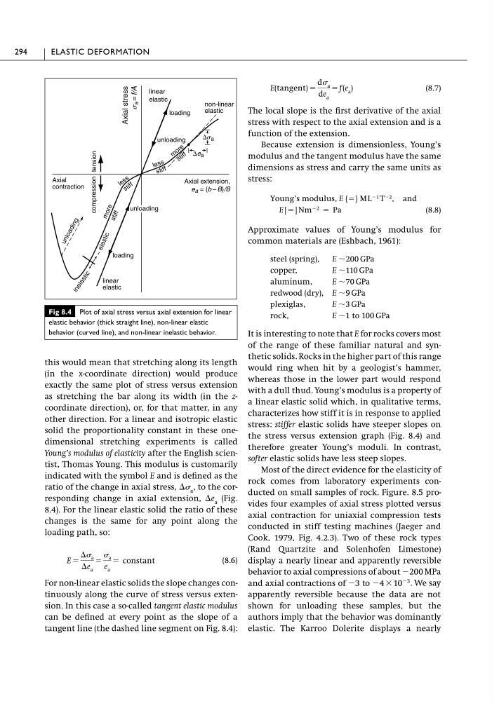
ratio of the change in axial stress, ⌬ a , to the corresponding change in axial extension, ⌬e a (Fig.
8.4). For the linear elastic solid the ratio of these
changes is the same for any point along the
loading path, so:
(8.6)
For non-linear elastic solids the slope changes continuously along the curve of stress versus extension. In this case a so-called tangent elastic modulus
can be defined at every point as the slope of a
tangent line (the dashed line segment on Fig. 8.4):
E ϭ
⌬ a
⌬e a
ϭ
a
e a
ϭ constant
(8.7)
The local slope is the first derivative of the axial
stress with respect to the axial extension and is a
function of the extension.
Because extension is dimensionless, Young’s
modulus and the tangent modulus have the same
dimensions as stress and carry the same units as
stress:
(8.8)
Approximate values of Young’s modulus for
common materials are (Eshbach, 1961):
steel (spring),
E ϳ200 GPa
copper,
E ϳ110 GPa
aluminum,
E ϳ70 GPa
redwood (dry), E ϳ9 GPa
plexiglas,
E ϳ3 GPa
rock,
E ϳ1 to 100 GPa
It is interesting to note that E for rocks covers most
of the range of these familiar natural and synthetic solids. Rocks in the higher part of this range
would ring when hit by a geologist’s hammer,
whereas those in the lower part would respond
with a dull thud. Young’s modulus is a property of
a linear elastic solid which, in qualitative terms,
characterizes how stiff it is in response to applied
stress: stiffer elastic solids have steeper slopes on
the stress versus extension graph (Fig. 8.4) and
therefore greater Young’s moduli. In contrast,
softer elastic solids have less steep slopes.
Most of the direct evidence for the elasticity of
rock comes from laboratory experiments conducted on small samples of rock. Figure. 8.5 provides four examples of axial stress plotted versus
axial contraction for uniaxial compression tests
conducted in stiff testing machines (Jaeger and
Cook, 1979, Fig. 4.2.3). Two of these rock types
(Rand Quartzite and Solenhofen Limestone)
display a nearly linear and apparently reversible
behavior to axial compressions of about Ϫ200 MPa
and axial contractions of Ϫ3 to Ϫ4 ϫ 10
Ϫ3 . We say
apparently reversible because the data are not
shown for unloading these samples, but the
authors imply that the behavior was dominantly
elastic. The Karroo Dolerite displays a nearly
E [ϭ] Nm Ϫ2 ϭ Pa
Young’s modulus, E {ϭ} M L Ϫ1 T Ϫ2 , and
E(tangent) ϭ
d a
de a
ϭ f (e a )
294
ELASTIC DEFORMATION
Fig 8.4 Plot of axial stress versus axial extension for linear
elastic behavior (thick straight line), non-linear elastic
behavior (curved line), and non-linear inelastic behavior.
m
o r e
s t if f
le s s
s ti ff
loading
non-linear
elastic
Axial extension,
e a = (b – B)/B
tension
compression
linear
elastic
in e la s t ic
~ e la s ti c
loading
Axial
contraction
le s s
s t if f
m o re
s ti ff
⌬e a
⌬s a
Axial stress
s
a =
f/A
linear
elastic
unloading
unloading
u n lo a d in g
(in the x-coordinate direction) would produce
exactly the same plot of stress versus extension
as stretching the bar along its width (in the zcoordinate direction), or, for that matter, in any
other direction. For a linear and isotropic elastic
solid the proportionality constant in these onedimensional stretching experiments is called
Young’s modulus of elasticity after the English scientist, Thomas Young. This modulus is customarily
indicated with the symbol E and is defined as the
ratio of the change in axial stress, ⌬ a , to the corresponding change in axial extension, ⌬e a (Fig.
8.4). For the linear elastic solid the ratio of these
changes is the same for any point along the
loading path, so:
(8.6)
For non-linear elastic solids the slope changes continuously along the curve of stress versus extension. In this case a so-called tangent elastic modulus
can be defined at every point as the slope of a
tangent line (the dashed line segment on Fig. 8.4):
E ϭ
⌬ a
⌬e a
ϭ
a
e a
ϭ constant
(8.7)
The local slope is the first derivative of the axial
stress with respect to the axial extension and is a
function of the extension.
Because extension is dimensionless, Young’s
modulus and the tangent modulus have the same
dimensions as stress and carry the same units as
stress:
(8.8)
Approximate values of Young’s modulus for
common materials are (Eshbach, 1961):
steel (spring),
E ϳ200 GPa
copper,
E ϳ110 GPa
aluminum,
E ϳ70 GPa
redwood (dry), E ϳ9 GPa
plexiglas,
E ϳ3 GPa
rock,
E ϳ1 to 100 GPa
It is interesting to note that E for rocks covers most
of the range of these familiar natural and synthetic solids. Rocks in the higher part of this range
would ring when hit by a geologist’s hammer,
whereas those in the lower part would respond
with a dull thud. Young’s modulus is a property of
a linear elastic solid which, in qualitative terms,
characterizes how stiff it is in response to applied
stress: stiffer elastic solids have steeper slopes on
the stress versus extension graph (Fig. 8.4) and
therefore greater Young’s moduli. In contrast,
softer elastic solids have less steep slopes.
Most of the direct evidence for the elasticity of
rock comes from laboratory experiments conducted on small samples of rock. Figure. 8.5 provides four examples of axial stress plotted versus
axial contraction for uniaxial compression tests
conducted in stiff testing machines (Jaeger and
Cook, 1979, Fig. 4.2.3). Two of these rock types
(Rand Quartzite and Solenhofen Limestone)
display a nearly linear and apparently reversible
behavior to axial compressions of about Ϫ200 MPa
and axial contractions of Ϫ3 to Ϫ4 ϫ 10
Ϫ3 . We say
apparently reversible because the data are not
shown for unloading these samples, but the
authors imply that the behavior was dominantly
elastic. The Karroo Dolerite displays a nearly
E [ϭ] Nm Ϫ2 ϭ Pa
Young’s modulus, E {ϭ} M L Ϫ1 T Ϫ2 , and
E(tangent) ϭ
d a
de a
ϭ f (e a )
294
ELASTIC DEFORMATION
Fig 8.4 Plot of axial stress versus axial extension for linear
elastic behavior (thick straight line), non-linear elastic
behavior (curved line), and non-linear inelastic behavior.
m
o r e
s t if f
le s s
s ti ff
loading
non-linear
elastic
Axial extension,
e a = (b – B)/B
tension
compression
linear
elastic
in e la s t ic
~ e la s ti c
loading
Axial
contraction
le s s
s t if f
m o re
s ti ff
⌬e a
⌬s a
Axial stress
s
a =
f/A
linear
elastic
unloading
unloading
u n lo a d in g