

tions to geology. The incomplete, one-dimensional
form of the elasticity model introduced by Hooke
was further developed in the 1700s by Bernoulli
and Euler in order to describe the deformation of
beams of materials used in construction. The
development of a complete model was impossible
at that time, because it depended on understanding the general concepts of stress and strain,
which were not formulated until 1822 by Cauchy
(Malvern, 1969).
We construct in our minds a perfectly elastic
solid, one for which the extension is completely
recoverable upon release of the stress. In order to
focus on mechanical relationships, the temperature is postulated to be constant, so we consider
isothermal conditions, and the bar is postulated to
have homogeneous material properties. To quantify
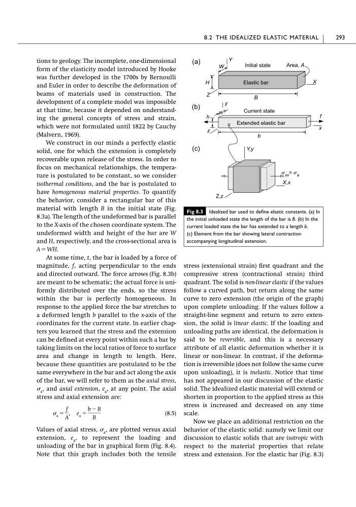
the behavior, consider a rectangular bar of this
material with length B in the initial state (Fig.
8.3a). The length of the undeformed bar is parallel
to the X-axis of the chosen coordinate system. The
undeformed width and height of the bar are W
and H, respectively, and the cross-sectional area is
A ϭ WH.
At some time, t, the bar is loaded by a force of
magnitude, f, acting perpendicular to the ends
and directed outward. The force arrows (Fig. 8.3b)
are meant to be schematic; the actual force is uniformly distributed over the ends, so the stress
within the bar is perfectly homogeneous. In
response to the applied force the bar stretches to
a deformed length b parallel to the x-axis of the
coordinates for the current state. In earlier chapters you learned that the stress and the extension
can be defined at every point within such a bar by
taking limits on the local ratios of force to surface
area and change in length to length. Here,
because these quantities are postulated to be the
same everywhere in the bar and act along the axis
of the bar, we will refer to them as the axial stress,
a , and axial extension, e a , at any point. The axial
stress and axial extension are:
(8.5)
Values of axial stress, a , are plotted versus axial
extension, e a , to represent the loading and
unloading of the bar in graphical form (Fig. 8.4).
Note that this graph includes both the tensile
a ϭ
f
A
, e a ϭ
b Ϫ B
B
stress (extensional strain) first quadrant and the
compressive stress (contractional strain) third
quadrant. The solid is non-linear elastic if the values
follow a curved path, but return along the same
curve to zero extension (the origin of the graph)
upon complete unloading. If the values follow a
straight-line segment and return to zero extension, the solid is linear elastic. If the loading and
unloading paths are identical, the deformation is
said to be reversible, and this is a necessary
attribute of all elastic deformation whether it is
linear or non-linear. In contrast, if the deformation is irreversible (does not follow the same curve
upon unloading), it is inelastic. Notice that time
has not appeared in our discussion of the elastic
solid. The idealized elastic material will extend or
shorten in proportion to the applied stress as this
stress is increased and decreased on any time
scale.
Now we place an additional restriction on the
behavior of the elastic solid: namely we limit our
discussion to elastic solids that are isotropic with
respect to the material properties that relate
stress and extension. For the elastic bar (Fig. 8.3)
8.2 THE IDEALIZED ELASTIC MATERIAL
293
Fig 8.3 Idealized bar used to define elastic constants. (a) In
the initial unloaded state the length of the bar is B. (b) In the
current loaded state the bar has extended to a length b.
(c) Element from the bar showing lateral contraction
accompanying longitudinal extension.
b
(a)
B
f
Elastic bar
(b)
Extended elastic bar
X,x
Y,y
Z,z
W
(c)
X
Y
Z
x
y
z
w
Area, A
H
Initial state
Current state
xx = a
h
form of the elasticity model introduced by Hooke
was further developed in the 1700s by Bernoulli
and Euler in order to describe the deformation of
beams of materials used in construction. The
development of a complete model was impossible
at that time, because it depended on understanding the general concepts of stress and strain,
which were not formulated until 1822 by Cauchy
(Malvern, 1969).
We construct in our minds a perfectly elastic
solid, one for which the extension is completely
recoverable upon release of the stress. In order to
focus on mechanical relationships, the temperature is postulated to be constant, so we consider
isothermal conditions, and the bar is postulated to
have homogeneous material properties. To quantify
the behavior, consider a rectangular bar of this
material with length B in the initial state (Fig.
8.3a). The length of the undeformed bar is parallel
to the X-axis of the chosen coordinate system. The
undeformed width and height of the bar are W
and H, respectively, and the cross-sectional area is
A ϭ WH.
At some time, t, the bar is loaded by a force of
magnitude, f, acting perpendicular to the ends
and directed outward. The force arrows (Fig. 8.3b)
are meant to be schematic; the actual force is uniformly distributed over the ends, so the stress
within the bar is perfectly homogeneous. In
response to the applied force the bar stretches to
a deformed length b parallel to the x-axis of the
coordinates for the current state. In earlier chapters you learned that the stress and the extension
can be defined at every point within such a bar by
taking limits on the local ratios of force to surface
area and change in length to length. Here,
because these quantities are postulated to be the
same everywhere in the bar and act along the axis
of the bar, we will refer to them as the axial stress,
a , and axial extension, e a , at any point. The axial
stress and axial extension are:
(8.5)
Values of axial stress, a , are plotted versus axial
extension, e a , to represent the loading and
unloading of the bar in graphical form (Fig. 8.4).
Note that this graph includes both the tensile
a ϭ
f
A
, e a ϭ
b Ϫ B
B
stress (extensional strain) first quadrant and the
compressive stress (contractional strain) third
quadrant. The solid is non-linear elastic if the values
follow a curved path, but return along the same
curve to zero extension (the origin of the graph)
upon complete unloading. If the values follow a
straight-line segment and return to zero extension, the solid is linear elastic. If the loading and
unloading paths are identical, the deformation is
said to be reversible, and this is a necessary
attribute of all elastic deformation whether it is
linear or non-linear. In contrast, if the deformation is irreversible (does not follow the same curve
upon unloading), it is inelastic. Notice that time
has not appeared in our discussion of the elastic
solid. The idealized elastic material will extend or
shorten in proportion to the applied stress as this
stress is increased and decreased on any time
scale.
Now we place an additional restriction on the
behavior of the elastic solid: namely we limit our
discussion to elastic solids that are isotropic with
respect to the material properties that relate
stress and extension. For the elastic bar (Fig. 8.3)
8.2 THE IDEALIZED ELASTIC MATERIAL
293
Fig 8.3 Idealized bar used to define elastic constants. (a) In
the initial unloaded state the length of the bar is B. (b) In the
current loaded state the bar has extended to a length b.
(c) Element from the bar showing lateral contraction
accompanying longitudinal extension.
b
(a)
B
f
Elastic bar
(b)
Extended elastic bar
X,x
Y,y
Z,z
W
(c)
X
Y
Z
x
y
z
w
Area, A
H
Initial state
Current state
xx = a
h