

The derivation of the compatibility equations
in terms of the stress components is given in
detail elsewhere (Malvern, 1969, p. 502). In short,
the stress components are substituted for the
strain components using (7.149) and the equilibrium equations (7.139) are used to simplify the
resulting equations and find the so-called
Beltrami–Michell compatibility equations for the
isothermal and isotropic linear elastic material.
In the most general form of these equations there
are partial derivatives of the body force per unit
volume with respect to the material coordinates.
To be consistent with our development thus far
the body force is taken as mass density times gravitational acceleration, g*, which is postulated to
be uniform in space and constant in time. Under
these conditions terms containing the body force
drop out of the Beltrami–Michell compatibility
equations which reduce to:
(7.151)
As mentioned above, these six equations represent only three independent conditions. These
compatibility equations and the equilibrium
equations (7.139) form a complete set for threedimensional problems in elastic theory where the
six stress components are the dependent variables.
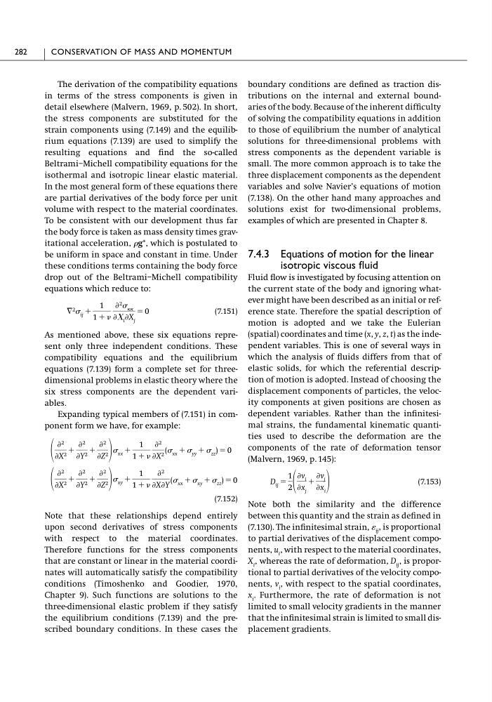
Expanding typical members of (7.151) in component form we have, for example:
(7.152)
Note that these relationships depend entirely
upon second derivatives of stress components
with respect to the material coordinates.
Therefore functions for the stress components
that are constant or linear in the material coordinates will automatically satisfy the compatibility
conditions (Timoshenko and Goodier, 1970,
Chapter 9). Such functions are solutions to the
three-dimensional elastic problem if they satisfy
the equilibrium conditions (7.139) and the prescribed boundary conditions. In these cases the
( xx ϩ xy ϩ zz ) ϭ 0
Ѩ 2
ѨX 2 ϩ
Ѩ 2
ѨY 2 ϩ
Ѩ 2
ѨZ 2 xy ϩ
1
1 ϩ
Ѩ 2
ѨXѨY
Ѩ 2
ѨX 2 ϩ
Ѩ 2
ѨY 2 ϩ
Ѩ 2
ѨZ 2 xx ϩ
1
1 ϩ
Ѩ 2
ѨX 2 ( xx ϩ yy ϩ zz ) ϭ 0
ٌ 2 ij ϩ
1
1 ϩ
Ѩ 2
Ѩ⌾ i ѨX j
ϭ 0
boundary conditions are defined as traction distributions on the internal and external boundaries of the body. Because of the inherent difficulty
of solving the compatibility equations in addition
to those of equilibrium the number of analytical
solutions for three-dimensional problems with
stress components as the dependent variable is
small. The more common approach is to take the
three displacement components as the dependent
variables and solve Navier’s equations of motion
(7.138). On the other hand many approaches and
solutions exist for two-dimensional problems,
examples of which are presented in Chapter 8.
7.4.3 Equations of motion for the linear
isotropic viscous fluid
Fluid flow is investigated by focusing attention on
the current state of the body and ignoring whatever might have been described as an initial or reference state. Therefore the spatial description of
motion is adopted and we take the Eulerian
(spatial) coordinates and time (x, y, z, t) as the independent variables. This is one of several ways in
which the analysis of fluids differs from that of
elastic solids, for which the referential description of motion is adopted. Instead of choosing the
displacement components of particles, the velocity components at given positions are chosen as
dependent variables. Rather than the infinitesimal strains, the fundamental kinematic quantities used to describe the deformation are the
components of the rate of deformation tensor
(Malvern, 1969, p. 145):
(7.153)
Note both the similarity and the difference
between this quantity and the strain as defined in
(7.130). The infinitesimal strain, ij , is proportional
to partial derivatives of the displacement components, u i , with respect to the material coordinates,
X i , whereas the rate of deformation, D ij , is proportional to partial derivatives of the velocity components, v i , with respect to the spatial coordinates,
x i . Furthermore, the rate of deformation is not
limited to small velocity gradients in the manner
that the infinitesimal strain is limited to small displacement gradients.
D ij ϭ
1
2
Ѩv i
Ѩx j
ϩ
Ѩv j
Ѩx i
282
CONSERVATION OF MASS AND MOMENTUM
in terms of the stress components is given in
detail elsewhere (Malvern, 1969, p. 502). In short,
the stress components are substituted for the
strain components using (7.149) and the equilibrium equations (7.139) are used to simplify the
resulting equations and find the so-called
Beltrami–Michell compatibility equations for the
isothermal and isotropic linear elastic material.
In the most general form of these equations there
are partial derivatives of the body force per unit
volume with respect to the material coordinates.
To be consistent with our development thus far
the body force is taken as mass density times gravitational acceleration, g*, which is postulated to
be uniform in space and constant in time. Under
these conditions terms containing the body force
drop out of the Beltrami–Michell compatibility
equations which reduce to:
(7.151)
As mentioned above, these six equations represent only three independent conditions. These
compatibility equations and the equilibrium
equations (7.139) form a complete set for threedimensional problems in elastic theory where the
six stress components are the dependent variables.
Expanding typical members of (7.151) in component form we have, for example:
(7.152)
Note that these relationships depend entirely
upon second derivatives of stress components
with respect to the material coordinates.
Therefore functions for the stress components
that are constant or linear in the material coordinates will automatically satisfy the compatibility
conditions (Timoshenko and Goodier, 1970,
Chapter 9). Such functions are solutions to the
three-dimensional elastic problem if they satisfy
the equilibrium conditions (7.139) and the prescribed boundary conditions. In these cases the
( xx ϩ xy ϩ zz ) ϭ 0
Ѩ 2
ѨX 2 ϩ
Ѩ 2
ѨY 2 ϩ
Ѩ 2
ѨZ 2 xy ϩ
1
1 ϩ
Ѩ 2
ѨXѨY
Ѩ 2
ѨX 2 ϩ
Ѩ 2
ѨY 2 ϩ
Ѩ 2
ѨZ 2 xx ϩ
1
1 ϩ
Ѩ 2
ѨX 2 ( xx ϩ yy ϩ zz ) ϭ 0
ٌ 2 ij ϩ
1
1 ϩ
Ѩ 2
Ѩ⌾ i ѨX j
ϭ 0
boundary conditions are defined as traction distributions on the internal and external boundaries of the body. Because of the inherent difficulty
of solving the compatibility equations in addition
to those of equilibrium the number of analytical
solutions for three-dimensional problems with
stress components as the dependent variable is
small. The more common approach is to take the
three displacement components as the dependent
variables and solve Navier’s equations of motion
(7.138). On the other hand many approaches and
solutions exist for two-dimensional problems,
examples of which are presented in Chapter 8.
7.4.3 Equations of motion for the linear
isotropic viscous fluid
Fluid flow is investigated by focusing attention on
the current state of the body and ignoring whatever might have been described as an initial or reference state. Therefore the spatial description of
motion is adopted and we take the Eulerian
(spatial) coordinates and time (x, y, z, t) as the independent variables. This is one of several ways in
which the analysis of fluids differs from that of
elastic solids, for which the referential description of motion is adopted. Instead of choosing the
displacement components of particles, the velocity components at given positions are chosen as
dependent variables. Rather than the infinitesimal strains, the fundamental kinematic quantities used to describe the deformation are the
components of the rate of deformation tensor
(Malvern, 1969, p. 145):
(7.153)
Note both the similarity and the difference
between this quantity and the strain as defined in
(7.130). The infinitesimal strain, ij , is proportional
to partial derivatives of the displacement components, u i , with respect to the material coordinates,
X i , whereas the rate of deformation, D ij , is proportional to partial derivatives of the velocity components, v i , with respect to the spatial coordinates,
x i . Furthermore, the rate of deformation is not
limited to small velocity gradients in the manner
that the infinitesimal strain is limited to small displacement gradients.
D ij ϭ
1
2
Ѩv i
Ѩx j
ϩ
Ѩv j
Ѩx i
282
CONSERVATION OF MASS AND MOMENTUM