

variables (unknowns) are the three displacement
components
A solution would be three
equations for the displacement components as
functions of the material coordinates and time.
The three equations, (7.135)–(7.137), are solved for
an elastic body of prescribed geometry subject to
boundary conditions defined at every point on the
exterior and interior boundaries in terms of the
three displacement components. Derivatives of
the displacement components with respect to
time provide the particle velocity as in (7.125) and
the particle acceleration as in (7.126). Derivatives
of the displacement components with respect to
the material coordinates (7.130) provide the infinitesimal strain components, and the isotropic
forms of Hooke’s Law (7.131) provide the stress
components. In this way all of the relevant physical quantities are accounted for as functions of
the material coordinates and time, and the fundamental laws of conservation of mass and
momentum are obeyed.
The most familiar applications of solutions to
the dynamic equations of elasticity (7.134) are to
bodies set in motion by sudden loading or unloading, for example from an explosion or the impact
of two bodies in motion, that generate waves
within the elastic solid (Achenbach, 1973), or from
the rapid propagation of a fracture (Freund, 1979).
Well-known geological examples include the
motion immediately following an explosive volcanic eruption, the impact of a meteor (Melosh,
1989), or the rupture of a fault (Li, 1987; Kostrov
and Das, 1988; Scholz, 1990). In these cases rock
particles close to the impulsive event are set in
motion first, while the rest of the body is unaffected. Seismic waves propagate outward from the
source with speeds on the order of a few kilometers per second and set the rest of the rock
mass in motion (Aki and Richards, 1980).
7.4.2 Quasi-static equilibrium for the
linear isotropic elastic solid
The equations of motion (7.134) for the isotropic
and isothermal linear elastic material place no
restrictions on the magnitudes of the velocity or
acceleration of any particle in the continuum.
They describe a material that may be accelerating
or decelerating, but these changes are always
related to the appropriate forces, so momentum is
(u x , u y , u z ).
conserved. Typically, however, the structural geologist is not confronted with data in the field that
directly constrain the particle velocity or acceleration. Rather it is the displacement from some
inferred initial configuration to the current
configuration, as in the opening of a dike or the
slip on a fault. Therefore, the structural geologist
generally approaches problems related to the
development of structures from a point of view in
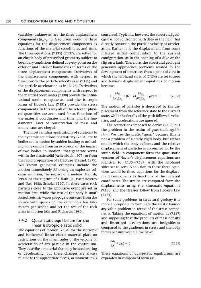
which the left-hand sides of (7.134) are set to zero
and Navier’s displacement equations of motion
become:
(7.138)
The motion of particles is described by the displacement from the reference state to the current
state, while the details of the path followed, velocities, and accelerations are ignored.
The restrictions imposed to derive (7.138) put
the problem in the realm of quasi-static equilibrium. We use the prefix “quasi” because this is
not a problem of a static rigid body, but rather
one in which the body deforms and the relative
displacement of particles is accounted for by the
strain field. In component form the quasi-static
versions of Navier’s displacement equations are
identical to (7.135)–(7.137) with the left-hand
sides set to zero. A solution to these three equations would be three equations for the displacement components as functions of the material
coordinates. The strains are computed from the
displacements using the kinematic equations
(7.130) and the stresses follow from Hooke’s Law
(7.131).
For some problems in structural geology it is
more appropriate to formulate the elastic boundary value problem in terms of the stress components. Taking the equations of motion as (7.127)
and supposing that the products of mass density
and linearized accelerations are insignificant
compared to the gradients in stress and the body
forces per unit volume, we have:
(7.139)
These equations of quasi-static equilibrium are
expanded in component form as:
Ѩ ji
ѨX j
ϩ g* i ϭ 0
G
Ѩ 2 u i
ѨX k ѨX k
ϩ (G ϩ )
Ѩ 2 u k
ѨX i ѨX k
ϩ g* i ϭ 0
280
CONSERVATION OF MASS AND MOMENTUM
components
A solution would be three
equations for the displacement components as
functions of the material coordinates and time.
The three equations, (7.135)–(7.137), are solved for
an elastic body of prescribed geometry subject to
boundary conditions defined at every point on the
exterior and interior boundaries in terms of the
three displacement components. Derivatives of
the displacement components with respect to
time provide the particle velocity as in (7.125) and
the particle acceleration as in (7.126). Derivatives
of the displacement components with respect to
the material coordinates (7.130) provide the infinitesimal strain components, and the isotropic
forms of Hooke’s Law (7.131) provide the stress
components. In this way all of the relevant physical quantities are accounted for as functions of
the material coordinates and time, and the fundamental laws of conservation of mass and
momentum are obeyed.
The most familiar applications of solutions to
the dynamic equations of elasticity (7.134) are to
bodies set in motion by sudden loading or unloading, for example from an explosion or the impact
of two bodies in motion, that generate waves
within the elastic solid (Achenbach, 1973), or from
the rapid propagation of a fracture (Freund, 1979).
Well-known geological examples include the
motion immediately following an explosive volcanic eruption, the impact of a meteor (Melosh,
1989), or the rupture of a fault (Li, 1987; Kostrov
and Das, 1988; Scholz, 1990). In these cases rock
particles close to the impulsive event are set in
motion first, while the rest of the body is unaffected. Seismic waves propagate outward from the
source with speeds on the order of a few kilometers per second and set the rest of the rock
mass in motion (Aki and Richards, 1980).
7.4.2 Quasi-static equilibrium for the
linear isotropic elastic solid
The equations of motion (7.134) for the isotropic
and isothermal linear elastic material place no
restrictions on the magnitudes of the velocity or
acceleration of any particle in the continuum.
They describe a material that may be accelerating
or decelerating, but these changes are always
related to the appropriate forces, so momentum is
(u x , u y , u z ).
conserved. Typically, however, the structural geologist is not confronted with data in the field that
directly constrain the particle velocity or acceleration. Rather it is the displacement from some
inferred initial configuration to the current
configuration, as in the opening of a dike or the
slip on a fault. Therefore, the structural geologist
generally approaches problems related to the
development of structures from a point of view in
which the left-hand sides of (7.134) are set to zero
and Navier’s displacement equations of motion
become:
(7.138)
The motion of particles is described by the displacement from the reference state to the current
state, while the details of the path followed, velocities, and accelerations are ignored.
The restrictions imposed to derive (7.138) put
the problem in the realm of quasi-static equilibrium. We use the prefix “quasi” because this is
not a problem of a static rigid body, but rather
one in which the body deforms and the relative
displacement of particles is accounted for by the
strain field. In component form the quasi-static
versions of Navier’s displacement equations are
identical to (7.135)–(7.137) with the left-hand
sides set to zero. A solution to these three equations would be three equations for the displacement components as functions of the material
coordinates. The strains are computed from the
displacements using the kinematic equations
(7.130) and the stresses follow from Hooke’s Law
(7.131).
For some problems in structural geology it is
more appropriate to formulate the elastic boundary value problem in terms of the stress components. Taking the equations of motion as (7.127)
and supposing that the products of mass density
and linearized accelerations are insignificant
compared to the gradients in stress and the body
forces per unit volume, we have:
(7.139)
These equations of quasi-static equilibrium are
expanded in component form as:
Ѩ ji
ѨX j
ϩ g* i ϭ 0
G
Ѩ 2 u i
ѨX k ѨX k
ϩ (G ϩ )
Ѩ 2 u k
ѨX i ѨX k
ϩ g* i ϭ 0
280
CONSERVATION OF MASS AND MOMENTUM