

The three equations of motion (7.127), six kinematic equations (7.130), and six constitutive equations (7.131) form a complete set of field equations
for the linearized isotropic and isothermal elastic
material. The independent variables are the three
material coordinates and time (X, Y, Z, t). The
dependent variables (unknowns) are the three displacement components
, the six infinitesimal strain components
, and
the six stress components
.
Usually, the mass density, , the components of
gravitational acceleration,
and the two elastic
constants, G and , are taken as given by laboratory or field data, and in most applications these
quantities are postulated to be uniform in space
and constant in time.
There are fifteen field equations and fifteen
unknowns for the elastic boundary value problem
as posed above. This problem is put in a more practical form by replacing the stress components in
(7.127) with displacement components using the
kinematic equations (7.130) and Hooke’s Law
(7.131), for example as:
(7.133)
The other stress components follow by similar
steps. Then (7.127) is written:
(7.134)
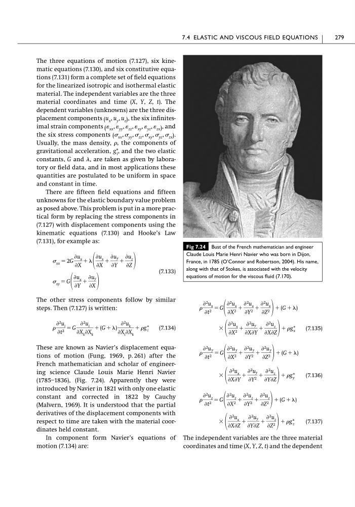
These are known as Navier’s displacement equations of motion (Fung, 1969, p. 261) after the
French mathematician and scholar of engineering science Claude Louis Marie Henri Navier
(1785–1836), (Fig. 7.24). Apparently they were
introduced by Navier in 1821 with only one elastic
constant and corrected in 1822 by Cauchy
(Malvern, 1969). It is understood that the partial
derivatives of the displacement components with
respect to time are taken with the material coordinates held constant.
In component form Navier’s equations of
motion (7.134) are:
Ѩ 2 u i
Ѩt 2 ϭ G
Ѩ 2 u i
ѨX k ѨX k
ϩ (G ϩ )
Ѩ 2 u k
ѨX i ѨX k
ϩ g* i
xy ϭ G
Ѩu x
ѨY
ϩ
Ѩu y
ѨX
xx ϭ 2G
Ѩu x
ѨX
ϩ
Ѩu x
ѨX
ϩ
Ѩu y
ѨY
ϩ
Ѩu z
ѨZ
g* i ,
( xx , yy , zz , xy , yz , zx )
( xx , yy , zz , xy , yz , zx)
( u x , u y , u z )
(7.135)
(7.136)
(7.137)
The independent variables are the three material
coordinates and time (X, Y, Z, t) and the dependent
ϫ
Ѩ 2 u x
ѨXѨZ
ϩ
Ѩ 2 u y
ѨYѨZ
ϩ
Ѩ 2 u z
ѨZ 2 ϩ g* z
Ѩ 2 u z
Ѩt 2 ϭ G
Ѩ 2 u z
ѨX 2 ϩ
Ѩ 2 u z
ѨY 2 ϩ
Ѩ 2 u z
ѨZ 2 ϩ (G ϩ )
ϫ
Ѩ 2 u x
ѨXѨY
ϩ
Ѩ 2 u y
ѨY 2 ϩ
Ѩ 2 u z
ѨYѨZ ϩ g* y
Ѩ 2 u y
Ѩt 2 ϭ G
Ѩ 2 u y
ѨX 2 ϩ
Ѩ 2 u y
ѨY 2 ϩ
Ѩ 2 u y
ѨZ 2 ϩ (G ϩ )
ϫ
Ѩ 2 u x
ѨX 2 ϩ
Ѩ 2 u y
ѨXѨY
ϩ
Ѩ 2 u z
ѨXѨZ ϩ g* x
Ѩ 2 u x
Ѩt 2 ϭ G
Ѩ 2 u x
ѨX 2 ϩ
Ѩ 2 u x
ѨY 2 ϩ
Ѩ 2 u x
ѨZ 2
ϩ (G ϩ )
7.4 ELASTIC AND VISCOUS FIELD EQUATIONS
279
Fig 7.24 Bust of the French mathematician and engineer
Claude Louis Marie Henri Navier who was born in Dijon,
France, in 1785 (O’Connor and Robertson, 2004). His name,
along with that of Stokes, is associated with the velocity
equations of motion for the viscous fluid (7.170).
for the linearized isotropic and isothermal elastic
material. The independent variables are the three
material coordinates and time (X, Y, Z, t). The
dependent variables (unknowns) are the three displacement components
, the six infinitesimal strain components
, and
the six stress components
.
Usually, the mass density, , the components of
gravitational acceleration,
and the two elastic
constants, G and , are taken as given by laboratory or field data, and in most applications these
quantities are postulated to be uniform in space
and constant in time.
There are fifteen field equations and fifteen
unknowns for the elastic boundary value problem
as posed above. This problem is put in a more practical form by replacing the stress components in
(7.127) with displacement components using the
kinematic equations (7.130) and Hooke’s Law
(7.131), for example as:
(7.133)
The other stress components follow by similar
steps. Then (7.127) is written:
(7.134)
These are known as Navier’s displacement equations of motion (Fung, 1969, p. 261) after the
French mathematician and scholar of engineering science Claude Louis Marie Henri Navier
(1785–1836), (Fig. 7.24). Apparently they were
introduced by Navier in 1821 with only one elastic
constant and corrected in 1822 by Cauchy
(Malvern, 1969). It is understood that the partial
derivatives of the displacement components with
respect to time are taken with the material coordinates held constant.
In component form Navier’s equations of
motion (7.134) are:
Ѩ 2 u i
Ѩt 2 ϭ G
Ѩ 2 u i
ѨX k ѨX k
ϩ (G ϩ )
Ѩ 2 u k
ѨX i ѨX k
ϩ g* i
xy ϭ G
Ѩu x
ѨY
ϩ
Ѩu y
ѨX
xx ϭ 2G
Ѩu x
ѨX
ϩ
Ѩu x
ѨX
ϩ
Ѩu y
ѨY
ϩ
Ѩu z
ѨZ
g* i ,
( xx , yy , zz , xy , yz , zx )
( xx , yy , zz , xy , yz , zx)
( u x , u y , u z )
(7.135)
(7.136)
(7.137)
The independent variables are the three material
coordinates and time (X, Y, Z, t) and the dependent
ϫ
Ѩ 2 u x
ѨXѨZ
ϩ
Ѩ 2 u y
ѨYѨZ
ϩ
Ѩ 2 u z
ѨZ 2 ϩ g* z
Ѩ 2 u z
Ѩt 2 ϭ G
Ѩ 2 u z
ѨX 2 ϩ
Ѩ 2 u z
ѨY 2 ϩ
Ѩ 2 u z
ѨZ 2 ϩ (G ϩ )
ϫ
Ѩ 2 u x
ѨXѨY
ϩ
Ѩ 2 u y
ѨY 2 ϩ
Ѩ 2 u z
ѨYѨZ ϩ g* y
Ѩ 2 u y
Ѩt 2 ϭ G
Ѩ 2 u y
ѨX 2 ϩ
Ѩ 2 u y
ѨY 2 ϩ
Ѩ 2 u y
ѨZ 2 ϩ (G ϩ )
ϫ
Ѩ 2 u x
ѨX 2 ϩ
Ѩ 2 u y
ѨXѨY
ϩ
Ѩ 2 u z
ѨXѨZ ϩ g* x
Ѩ 2 u x
Ѩt 2 ϭ G
Ѩ 2 u x
ѨX 2 ϩ
Ѩ 2 u x
ѨY 2 ϩ
Ѩ 2 u x
ѨZ 2
ϩ (G ϩ )
7.4 ELASTIC AND VISCOUS FIELD EQUATIONS
279
Fig 7.24 Bust of the French mathematician and engineer
Claude Louis Marie Henri Navier who was born in Dijon,
France, in 1785 (O’Connor and Robertson, 2004). His name,
along with that of Stokes, is associated with the velocity
equations of motion for the viscous fluid (7.170).