

with those mentioned above. The general equation for the finite strain tensor using the referential description of motion is (Malvern, 1969,
p. 160):
(7.128)
The E ij are referred to as the Lagrangian finite
strain components, because the partial derivatives are taken with respect to the Lagrangian
(material) coordinates, X i , and this description of
motion is associated with Joseph-Louis Lagrange
(Fig. 7.14). Particular longitudinal and shear components of the strain tensor are linearized to find
the corresponding infinitesimal strain components, for example, as follows:
(7.129)
Note that the non-linear terms are products of the
displacement gradients and these must be small
compared to the displacement gradients themselves. With approximations such as these the
infinitesimal strain tensor, ij , is related to the displacement gradients as:
(7.130)
A finite strain tensor also may be written using
the spatial description of motion and when a
similar linearization is carried out an equation of
the same form as (7.130) emerges in which the
partial derivatives are taken with respect to the
Eulerian (spatial) coordinates, x i . Typically, the
distinction between these two descriptions of the
kinematics is overlooked in applications of linear
elasticity.
For the linear elastic material the stress components are related to the infinitesimal strain
components using constitutive equations called
Hooke’s Law after Robert Hooke (Fig. 7.23) the
English polymath and contemporary of Isaac
ij ϭ
1
2
Ѩu i
ѨX j
ϩ
Ѩu j
ѨX i
Ϸ
1
2
Ѩu x
ѨY
ϩ
Ѩu y
ѨX
E xy ϭ
1
2
Ѩu x
ѨY
ϩ
Ѩu y
ѨX
ϩ
1
2
Ѩu x
ѨX
Ѩu x
ѨY
ϩ
Ѩu y
ѨX
Ѩu y
ѨY
ϩ
Ѩu z
ѨX
Ѩu z
ѨY
E xx ϭ
Ѩu x
ѨX
ϩ
1
2 ΄
Ѩu x
ѨX
2
ϩ
Ѩuy
ѨX
2
ϩ
Ѩu z
ѨX
2
΅ Ϸ
Ѩu x
ѨX
E ij ϭ
1
2
Ѩu i
ѨX j
ϩ
Ѩu j
ѨX i
ϩ
Ѩu k
ѨX i
Ѩu k
ѨX j
Newton. Chapter 8 is devoted to a discussion of the
measurement of elastic material properties and
various forms of Hooke’s Law. The general linear
form is simplified here for an isotropic material:
one in which the elastic constants are not dependent upon direction. For such a material the
stress–strain relationships are:
(7.131)
Here G is the elastic shear modulus and is Lamé’s
constant. These are properties of the material and
they have the same units and dimensions as
stress. Expanding (7.131), typical normal and
shear components of stress are related to the
infinitesimal strains as:
(7.132)
xy ϭ 2G xy
xx ϭ 2G xx ϩ ( xx ϩ yy ϩ zz )
ij ϭ 2G ij ϩ kk ␦ ij
278
CONSERVATION OF MASS AND MOMENTUM
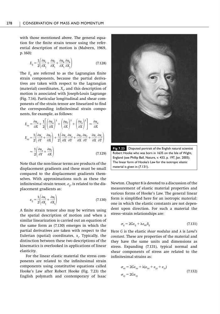
Fig 7.23 Disputed portrait of the English natural scientist
Robert Hooke who was born in 1635 on the Isle of Wight,
England (see Phillip Ball, Nature, v. 433, p. 197, Jan. 2005).
The linear form of Hooke’s Law for the isotropic elastic
material is given in (7.131).
p. 160):
(7.128)
The E ij are referred to as the Lagrangian finite
strain components, because the partial derivatives are taken with respect to the Lagrangian
(material) coordinates, X i , and this description of
motion is associated with Joseph-Louis Lagrange
(Fig. 7.14). Particular longitudinal and shear components of the strain tensor are linearized to find
the corresponding infinitesimal strain components, for example, as follows:
(7.129)
Note that the non-linear terms are products of the
displacement gradients and these must be small
compared to the displacement gradients themselves. With approximations such as these the
infinitesimal strain tensor, ij , is related to the displacement gradients as:
(7.130)
A finite strain tensor also may be written using
the spatial description of motion and when a
similar linearization is carried out an equation of
the same form as (7.130) emerges in which the
partial derivatives are taken with respect to the
Eulerian (spatial) coordinates, x i . Typically, the
distinction between these two descriptions of the
kinematics is overlooked in applications of linear
elasticity.
For the linear elastic material the stress components are related to the infinitesimal strain
components using constitutive equations called
Hooke’s Law after Robert Hooke (Fig. 7.23) the
English polymath and contemporary of Isaac
ij ϭ
1
2
Ѩu i
ѨX j
ϩ
Ѩu j
ѨX i
Ϸ
1
2
Ѩu x
ѨY
ϩ
Ѩu y
ѨX
E xy ϭ
1
2
Ѩu x
ѨY
ϩ
Ѩu y
ѨX
ϩ
1
2
Ѩu x
ѨX
Ѩu x
ѨY
ϩ
Ѩu y
ѨX
Ѩu y
ѨY
ϩ
Ѩu z
ѨX
Ѩu z
ѨY
E xx ϭ
Ѩu x
ѨX
ϩ
1
2 ΄
Ѩu x
ѨX
2
ϩ
Ѩuy
ѨX
2
ϩ
Ѩu z
ѨX
2
΅ Ϸ
Ѩu x
ѨX
E ij ϭ
1
2
Ѩu i
ѨX j
ϩ
Ѩu j
ѨX i
ϩ
Ѩu k
ѨX i
Ѩu k
ѨX j
Newton. Chapter 8 is devoted to a discussion of the
measurement of elastic material properties and
various forms of Hooke’s Law. The general linear
form is simplified here for an isotropic material:
one in which the elastic constants are not dependent upon direction. For such a material the
stress–strain relationships are:
(7.131)
Here G is the elastic shear modulus and is Lamé’s
constant. These are properties of the material and
they have the same units and dimensions as
stress. Expanding (7.131), typical normal and
shear components of stress are related to the
infinitesimal strains as:
(7.132)
xy ϭ 2G xy
xx ϭ 2G xx ϩ ( xx ϩ yy ϩ zz )
ij ϭ 2G ij ϩ kk ␦ ij
278
CONSERVATION OF MASS AND MOMENTUM
Fig 7.23 Disputed portrait of the English natural scientist
Robert Hooke who was born in 1635 on the Isle of Wight,
England (see Phillip Ball, Nature, v. 433, p. 197, Jan. 2005).
The linear form of Hooke’s Law for the isotropic elastic
material is given in (7.131).