

(7.75)
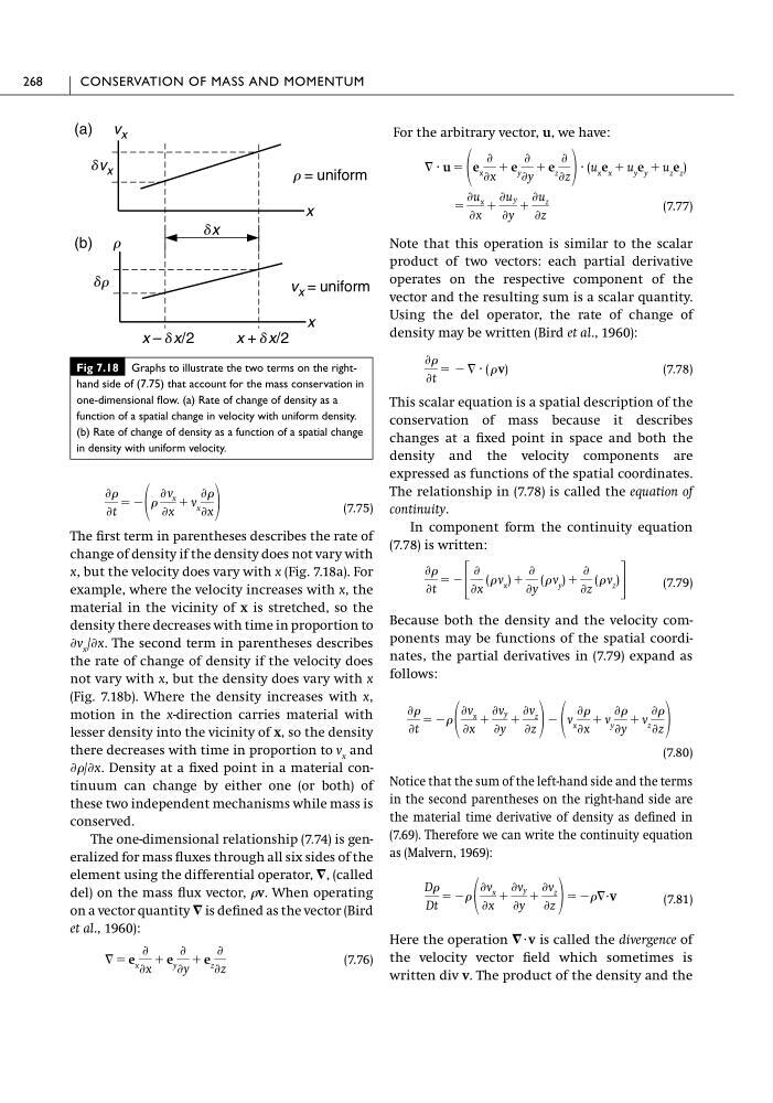
The first term in parentheses describes the rate of
change of density if the density does not vary with
x, but the velocity does vary with x (Fig. 7.18a). For
example, where the velocity increases with x, the
material in the vicinity of x is stretched, so the
density there decreases with time in proportion to
Ѩv x /Ѩx. The second term in parentheses describes
the rate of change of density if the velocity does
not vary with x, but the density does vary with x
(Fig. 7.18b). Where the density increases with x,
motion in the x-direction carries material with
lesser density into the vicinity of x, so the density
there decreases with time in proportion to v x and
Ѩ/Ѩx. Density at a fixed point in a material continuum can change by either one (or both) of
these two independent mechanisms while mass is
conserved.
The one-dimensional relationship (7.74) is generalized for mass fluxes through all six sides of the
element using the differential operator, ١, (called
del) on the mass flux vector, v. When operating
on a vector quantity ١ is defined as the vector (Bird
et al., 1960):
(7.76)
ٌ ϭ e x
Ѩ
Ѩx
ϩ e y
Ѩ
Ѩy
ϩ e z
Ѩ
Ѩz
Ѩ
Ѩt
ϭ Ϫ
Ѩv x
Ѩx
ϩ v x
Ѩ
Ѩx
For the arbitrary vector, u, we have:
(7.77)
Note that this operation is similar to the scalar
product of two vectors: each partial derivative
operates on the respective component of the
vector and the resulting sum is a scalar quantity.
Using the del operator, the rate of change of
density may be written (Bird et al., 1960):
(7.78)
This scalar equation is a spatial description of the
conservation of mass because it describes
changes at a fixed point in space and both the
density and the velocity components are
expressed as functions of the spatial coordinates.
The relationship in (7.78) is called the equation of
continuity.
In component form the continuity equation
(7.78) is written:
(7.79)
Because both the density and the velocity components may be functions of the spatial coordinates, the partial derivatives in (7.79) expand as
follows:
(7.80)
Notice that the sum of the left-hand side and the terms
in the second parentheses on the right-hand side are
the material time derivative of density as defined in
(7.69). Therefore we can write the continuity equation
as (Malvern, 1969):
ٌиv
(7.81)
Here the operation ١иv is called the divergence of
the velocity vector field which sometimes is
written div v. The product of the density and the
D
Dt
ϭ Ϫ
Ѩv x
Ѩx
ϩ
Ѩv y
Ѩy
ϩ
Ѩv z
Ѩz ϭ Ϫ
Ѩ
Ѩt
ϭ Ϫ
Ѩv x
Ѩx
ϩ
Ѩv y
Ѩy
ϩ
Ѩv z
Ѩz Ϫ v x
Ѩ
Ѩx
ϩ v y
Ѩ
Ѩy
ϩ v z
Ѩ
Ѩz
Ѩ
Ѩt
ϭ Ϫ
΄
Ѩ
Ѩx
( v x ) ϩ
Ѩ
Ѩy
( v y ) ϩ
Ѩ
Ѩz
( v z ) ΅
Ѩ
Ѩt
ϭ Ϫ ٌ · ( v)
ϭ
Ѩu x
Ѩx
ϩ
Ѩuy
Ѩy
ϩ
Ѩu z
Ѩz
ٌ · u ϭ
e x
Ѩ
Ѩx
ϩ e y
Ѩ
Ѩy
ϩ e z
Ѩ
Ѩz
· (u x e x ϩ u y e y ϩ u z e z )
268
CONSERVATION OF MASS AND MOMENTUM
Fig 7.18 Graphs to illustrate the two terms on the righthand side of (7.75) that account for the mass conservation in
one-dimensional flow. (a) Rate of change of density as a
function of a spatial change in velocity with uniform density.
(b) Rate of change of density as a function of a spatial change
in density with uniform velocity.
x
r
x
dx
v x
dv x
r = uniform
dr
v x = uniform
x – dx/2
x + dx/2
(a)
(b)
The first term in parentheses describes the rate of
change of density if the density does not vary with
x, but the velocity does vary with x (Fig. 7.18a). For
example, where the velocity increases with x, the
material in the vicinity of x is stretched, so the
density there decreases with time in proportion to
Ѩv x /Ѩx. The second term in parentheses describes
the rate of change of density if the velocity does
not vary with x, but the density does vary with x
(Fig. 7.18b). Where the density increases with x,
motion in the x-direction carries material with
lesser density into the vicinity of x, so the density
there decreases with time in proportion to v x and
Ѩ/Ѩx. Density at a fixed point in a material continuum can change by either one (or both) of
these two independent mechanisms while mass is
conserved.
The one-dimensional relationship (7.74) is generalized for mass fluxes through all six sides of the
element using the differential operator, ١, (called
del) on the mass flux vector, v. When operating
on a vector quantity ١ is defined as the vector (Bird
et al., 1960):
(7.76)
ٌ ϭ e x
Ѩ
Ѩx
ϩ e y
Ѩ
Ѩy
ϩ e z
Ѩ
Ѩz
Ѩ
Ѩt
ϭ Ϫ
Ѩv x
Ѩx
ϩ v x
Ѩ
Ѩx
For the arbitrary vector, u, we have:
(7.77)
Note that this operation is similar to the scalar
product of two vectors: each partial derivative
operates on the respective component of the
vector and the resulting sum is a scalar quantity.
Using the del operator, the rate of change of
density may be written (Bird et al., 1960):
(7.78)
This scalar equation is a spatial description of the
conservation of mass because it describes
changes at a fixed point in space and both the
density and the velocity components are
expressed as functions of the spatial coordinates.
The relationship in (7.78) is called the equation of
continuity.
In component form the continuity equation
(7.78) is written:
(7.79)
Because both the density and the velocity components may be functions of the spatial coordinates, the partial derivatives in (7.79) expand as
follows:
(7.80)
Notice that the sum of the left-hand side and the terms
in the second parentheses on the right-hand side are
the material time derivative of density as defined in
(7.69). Therefore we can write the continuity equation
as (Malvern, 1969):
ٌиv
(7.81)
Here the operation ١иv is called the divergence of
the velocity vector field which sometimes is
written div v. The product of the density and the
D
Dt
ϭ Ϫ
Ѩv x
Ѩx
ϩ
Ѩv y
Ѩy
ϩ
Ѩv z
Ѩz ϭ Ϫ
Ѩ
Ѩt
ϭ Ϫ
Ѩv x
Ѩx
ϩ
Ѩv y
Ѩy
ϩ
Ѩv z
Ѩz Ϫ v x
Ѩ
Ѩx
ϩ v y
Ѩ
Ѩy
ϩ v z
Ѩ
Ѩz
Ѩ
Ѩt
ϭ Ϫ
΄
Ѩ
Ѩx
( v x ) ϩ
Ѩ
Ѩy
( v y ) ϩ
Ѩ
Ѩz
( v z ) ΅
Ѩ
Ѩt
ϭ Ϫ ٌ · ( v)
ϭ
Ѩu x
Ѩx
ϩ
Ѩuy
Ѩy
ϩ
Ѩu z
Ѩz
ٌ · u ϭ
e x
Ѩ
Ѩx
ϩ e y
Ѩ
Ѩy
ϩ e z
Ѩ
Ѩz
· (u x e x ϩ u y e y ϩ u z e z )
268
CONSERVATION OF MASS AND MOMENTUM
Fig 7.18 Graphs to illustrate the two terms on the righthand side of (7.75) that account for the mass conservation in
one-dimensional flow. (a) Rate of change of density as a
function of a spatial change in velocity with uniform density.
(b) Rate of change of density as a function of a spatial change
in density with uniform velocity.
x
r
x
dx
v x
dv x
r = uniform
dr
v x = uniform
x – dx/2
x + dx/2
(a)
(b)