

Here the subscript after the vertical bar indicates
x also is a function of the independent variable X,
which is held constant during partial differentiation with respect to time. The material coordinates are held constant because we want to track
the velocity of a particular particle. For this
reason the partial derivative in (7.58) is referred to
as the material time derivative and the resulting
velocity is called the particle velocity (Malvern,
1969). To understand this viewpoint an analogy is
drawn to an observer, stationed at the origin of
the material coordinates (X, Y) in Fig. 7.13, who
measures the time rate of change of the particle at
every position along its path from X to x as the
fault slips.
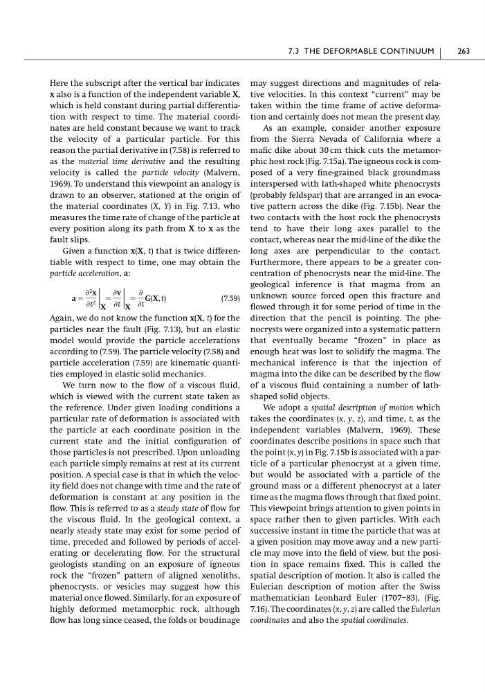
Given a function x(X, t) that is twice differentiable with respect to time, one may obtain the
particle acceleration, a:
(7.59)
Again, we do not know the function x(X, t) for the
particles near the fault (Fig. 7.13), but an elastic
model would provide the particle accelerations
according to (7.59). The particle velocity (7.58) and
particle acceleration (7.59) are kinematic quantities employed in elastic solid mechanics.
We turn now to the flow of a viscous fluid,
which is viewed with the current state taken as
the reference. Under given loading conditions a
particular rate of deformation is associated with
the particle at each coordinate position in the
current state and the initial configuration of
those particles is not prescribed. Upon unloading
each particle simply remains at rest at its current
position. A special case is that in which the velocity field does not change with time and the rate of
deformation is constant at any position in the
flow. This is referred to as a steady state of flow for
the viscous fluid. In the geological context, a
nearly steady state may exist for some period of
time, preceded and followed by periods of accelerating or decelerating flow. For the structural
geologists standing on an exposure of igneous
rock the “frozen” pattern of aligned xenoliths,
phenocrysts, or vesicles may suggest how this
material once flowed. Similarly, for an exposure of
highly deformed metamorphic rock, although
flow has long since ceased, the folds or boudinage
a ϭ
Ѩ 2 x
Ѩt 2 | X
ϭ
Ѩv
Ѩt | X
ϭ
Ѩ
Ѩt
G(X, t)
may suggest directions and magnitudes of relative velocities. In this context “current” may be
taken within the time frame of active deformation and certainly does not mean the present day.
As an example, consider another exposure
from the Sierra Nevada of California where a
mafic dike about 30 cm thick cuts the metamorphic host rock (Fig. 7.15a). The igneous rock is composed of a very fine-grained black groundmass
interspersed with lath-shaped white phenocrysts
(probably feldspar) that are arranged in an evocative pattern across the dike (Fig. 7.15b). Near the
two contacts with the host rock the phenocrysts
tend to have their long axes parallel to the
contact, whereas near the mid-line of the dike the
long axes are perpendicular to the contact.
Furthermore, there appears to be a greater concentration of phenocrysts near the mid-line. The
geological inference is that magma from an
unknown source forced open this fracture and
flowed through it for some period of time in the
direction that the pencil is pointing. The phenocrysts were organized into a systematic pattern
that eventually became “frozen” in place as
enough heat was lost to solidify the magma. The
mechanical inference is that the injection of
magma into the dike can be described by the flow
of a viscous fluid containing a number of lathshaped solid objects.
We adopt a spatial description of motion which
takes the coordinates (x, y, z), and time, t, as the
independent variables (Malvern, 1969). These
coordinates describe positions in space such that
the point (x, y) in Fig. 7.15b is associated with a particle of a particular phenocryst at a given time,
but would be associated with a particle of the
ground mass or a different phenocryst at a later
time as the magma flows through that fixed point.
This viewpoint brings attention to given points in
space rather then to given particles. With each
successive instant in time the particle that was at
a given position may move away and a new particle may move into the field of view, but the position in space remains fixed. This is called the
spatial description of motion. It also is called the
Eulerian description of motion after the Swiss
mathematician Leonhard Euler (1707–83), (Fig.
7.16). The coordinates (x, y, z) are called the Eulerian
coordinates and also the spatial coordinates.
7.3 THE DEFORMABLE CONTINUUM
263
x also is a function of the independent variable X,
which is held constant during partial differentiation with respect to time. The material coordinates are held constant because we want to track
the velocity of a particular particle. For this
reason the partial derivative in (7.58) is referred to
as the material time derivative and the resulting
velocity is called the particle velocity (Malvern,
1969). To understand this viewpoint an analogy is
drawn to an observer, stationed at the origin of
the material coordinates (X, Y) in Fig. 7.13, who
measures the time rate of change of the particle at
every position along its path from X to x as the
fault slips.
Given a function x(X, t) that is twice differentiable with respect to time, one may obtain the
particle acceleration, a:
(7.59)
Again, we do not know the function x(X, t) for the
particles near the fault (Fig. 7.13), but an elastic
model would provide the particle accelerations
according to (7.59). The particle velocity (7.58) and
particle acceleration (7.59) are kinematic quantities employed in elastic solid mechanics.
We turn now to the flow of a viscous fluid,
which is viewed with the current state taken as
the reference. Under given loading conditions a
particular rate of deformation is associated with
the particle at each coordinate position in the
current state and the initial configuration of
those particles is not prescribed. Upon unloading
each particle simply remains at rest at its current
position. A special case is that in which the velocity field does not change with time and the rate of
deformation is constant at any position in the
flow. This is referred to as a steady state of flow for
the viscous fluid. In the geological context, a
nearly steady state may exist for some period of
time, preceded and followed by periods of accelerating or decelerating flow. For the structural
geologists standing on an exposure of igneous
rock the “frozen” pattern of aligned xenoliths,
phenocrysts, or vesicles may suggest how this
material once flowed. Similarly, for an exposure of
highly deformed metamorphic rock, although
flow has long since ceased, the folds or boudinage
a ϭ
Ѩ 2 x
Ѩt 2 | X
ϭ
Ѩv
Ѩt | X
ϭ
Ѩ
Ѩt
G(X, t)
may suggest directions and magnitudes of relative velocities. In this context “current” may be
taken within the time frame of active deformation and certainly does not mean the present day.
As an example, consider another exposure
from the Sierra Nevada of California where a
mafic dike about 30 cm thick cuts the metamorphic host rock (Fig. 7.15a). The igneous rock is composed of a very fine-grained black groundmass
interspersed with lath-shaped white phenocrysts
(probably feldspar) that are arranged in an evocative pattern across the dike (Fig. 7.15b). Near the
two contacts with the host rock the phenocrysts
tend to have their long axes parallel to the
contact, whereas near the mid-line of the dike the
long axes are perpendicular to the contact.
Furthermore, there appears to be a greater concentration of phenocrysts near the mid-line. The
geological inference is that magma from an
unknown source forced open this fracture and
flowed through it for some period of time in the
direction that the pencil is pointing. The phenocrysts were organized into a systematic pattern
that eventually became “frozen” in place as
enough heat was lost to solidify the magma. The
mechanical inference is that the injection of
magma into the dike can be described by the flow
of a viscous fluid containing a number of lathshaped solid objects.
We adopt a spatial description of motion which
takes the coordinates (x, y, z), and time, t, as the
independent variables (Malvern, 1969). These
coordinates describe positions in space such that
the point (x, y) in Fig. 7.15b is associated with a particle of a particular phenocryst at a given time,
but would be associated with a particle of the
ground mass or a different phenocryst at a later
time as the magma flows through that fixed point.
This viewpoint brings attention to given points in
space rather then to given particles. With each
successive instant in time the particle that was at
a given position may move away and a new particle may move into the field of view, but the position in space remains fixed. This is called the
spatial description of motion. It also is called the
Eulerian description of motion after the Swiss
mathematician Leonhard Euler (1707–83), (Fig.
7.16). The coordinates (x, y, z) are called the Eulerian
coordinates and also the spatial coordinates.
7.3 THE DEFORMABLE CONTINUUM
263