

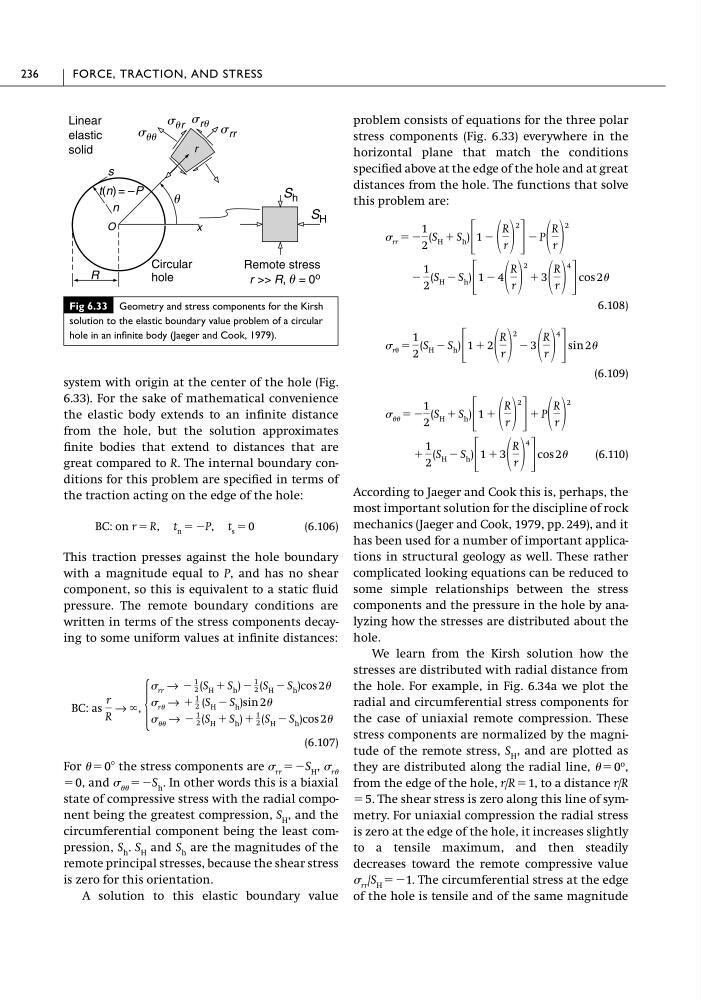
system with origin at the center of the hole (Fig.
6.33). For the sake of mathematical convenience
the elastic body extends to an infinite distance
from the hole, but the solution approximates
finite bodies that extend to distances that are
great compared to R. The internal boundary conditions for this problem are specified in terms of
the traction acting on the edge of the hole:
(6.106)
This traction presses against the hole boundary
with a magnitude equal to P, and has no shear
component, so this is equivalent to a static fluid
pressure. The remote boundary conditions are
written in terms of the stress components decaying to some uniform values at infinite distances:
(6.107)
For ϭ 0Њ the stress components are rr ϭϪS H , r
ϭ 0, and ϭϪS h . In other words this is a biaxial
state of compressive stress with the radial component being the greatest compression, S H , and the
circumferential component being the least compression, S h . S H and S h are the magnitudes of the
remote principal stresses, because the shear stress
is zero for this orientation.
A solution to this elastic boundary value
BC: as
r
R
→ ϱ,
Ά
rr → Ϫ
1
2 (S H ϩ S h ) Ϫ
1
2 (S H Ϫ S h )cos 2
r → ϩ
1
2 (S H Ϫ S h )sin 2
→ Ϫ
1
2 (S H ϩ S h ) ϩ
1
2 (S H Ϫ S h )cos 2
BC: on r ϭ R, t n ϭ ϪP, t s ϭ 0
problem consists of equations for the three polar
stress components (Fig. 6.33) everywhere in the
horizontal plane that match the conditions
specified above at the edge of the hole and at great
distances from the hole. The functions that solve
this problem are:
6.108)
(6.109)
(6.110)
According to Jaeger and Cook this is, perhaps, the
most important solution for the discipline of rock
mechanics (Jaeger and Cook, 1979, pp. 249), and it
has been used for a number of important applications in structural geology as well. These rather
complicated looking equations can be reduced to
some simple relationships between the stress
components and the pressure in the hole by analyzing how the stresses are distributed about the
hole.
We learn from the Kirsh solution how the
stresses are distributed with radial distance from
the hole. For example, in Fig. 6.34a we plot the
radial and circumferential stress components for
the case of uniaxial remote compression. These
stress components are normalized by the magnitude of the remote stress, S H , and are plotted as
they are distributed along the radial line, ϭ 0
o
,
from the edge of the hole, r/R ϭ 1, to a distance r/R
ϭ 5. The shear stress is zero along this line of symmetry. For uniaxial compression the radial stress
is zero at the edge of the hole, it increases slightly
to a tensile maximum, and then steadily
decreases toward the remote compressive value
rr /S H ϭϪ1. The circumferential stress at the edge
of the hole is tensile and of the same magnitude
ϩ
1
2
(S H Ϫ S h ) ΄ 1 ϩ 3
R
r
4
΅ cos 2
ϭ Ϫ
1
2
(S H ϩ S h )
΄
1 ϩ
R
r
2
΅
ϩ P
R
r
2
r ϭ
1
2
(S H Ϫ S h )
΄
1 ϩ 2
R
r
2
Ϫ 3
R
r
4
΅
sin 2
Ϫ
1
2
(S H Ϫ S h ) ΄ 1 Ϫ 4
R
r
2
ϩ 3
R
r
4
΅ cos 2
rr ϭ Ϫ
1
2
(S H ϩ S h )
΄
1 Ϫ
R
r
2
΅
Ϫ P
R
r
2
236
FORCE, TRACTION, AND STRESS
Fig 6.33 Geometry and stress components for the Kirsh
solution to the elastic boundary value problem of a circular
hole in an infinite body (Jaeger and Cook, 1979).
s uu
x
O
r
u
s
n
R
Circular
hole
Linear
elastic
solid
Remote stress
s ur s ru s rr
t(n) = –P
r >> R, u = 0 o
S h
S H
6.33). For the sake of mathematical convenience
the elastic body extends to an infinite distance
from the hole, but the solution approximates
finite bodies that extend to distances that are
great compared to R. The internal boundary conditions for this problem are specified in terms of
the traction acting on the edge of the hole:
(6.106)
This traction presses against the hole boundary
with a magnitude equal to P, and has no shear
component, so this is equivalent to a static fluid
pressure. The remote boundary conditions are
written in terms of the stress components decaying to some uniform values at infinite distances:
(6.107)
For ϭ 0Њ the stress components are rr ϭϪS H , r
ϭ 0, and ϭϪS h . In other words this is a biaxial
state of compressive stress with the radial component being the greatest compression, S H , and the
circumferential component being the least compression, S h . S H and S h are the magnitudes of the
remote principal stresses, because the shear stress
is zero for this orientation.
A solution to this elastic boundary value
BC: as
r
R
→ ϱ,
Ά
rr → Ϫ
1
2 (S H ϩ S h ) Ϫ
1
2 (S H Ϫ S h )cos 2
r → ϩ
1
2 (S H Ϫ S h )sin 2
→ Ϫ
1
2 (S H ϩ S h ) ϩ
1
2 (S H Ϫ S h )cos 2
BC: on r ϭ R, t n ϭ ϪP, t s ϭ 0
problem consists of equations for the three polar
stress components (Fig. 6.33) everywhere in the
horizontal plane that match the conditions
specified above at the edge of the hole and at great
distances from the hole. The functions that solve
this problem are:
6.108)
(6.109)
(6.110)
According to Jaeger and Cook this is, perhaps, the
most important solution for the discipline of rock
mechanics (Jaeger and Cook, 1979, pp. 249), and it
has been used for a number of important applications in structural geology as well. These rather
complicated looking equations can be reduced to
some simple relationships between the stress
components and the pressure in the hole by analyzing how the stresses are distributed about the
hole.
We learn from the Kirsh solution how the
stresses are distributed with radial distance from
the hole. For example, in Fig. 6.34a we plot the
radial and circumferential stress components for
the case of uniaxial remote compression. These
stress components are normalized by the magnitude of the remote stress, S H , and are plotted as
they are distributed along the radial line, ϭ 0
o
,
from the edge of the hole, r/R ϭ 1, to a distance r/R
ϭ 5. The shear stress is zero along this line of symmetry. For uniaxial compression the radial stress
is zero at the edge of the hole, it increases slightly
to a tensile maximum, and then steadily
decreases toward the remote compressive value
rr /S H ϭϪ1. The circumferential stress at the edge
of the hole is tensile and of the same magnitude
ϩ
1
2
(S H Ϫ S h ) ΄ 1 ϩ 3
R
r
4
΅ cos 2
ϭ Ϫ
1
2
(S H ϩ S h )
΄
1 ϩ
R
r
2
΅
ϩ P
R
r
2
r ϭ
1
2
(S H Ϫ S h )
΄
1 ϩ 2
R
r
2
Ϫ 3
R
r
4
΅
sin 2
Ϫ
1
2
(S H Ϫ S h ) ΄ 1 Ϫ 4
R
r
2
ϩ 3
R
r
4
΅ cos 2
rr ϭ Ϫ
1
2
(S H ϩ S h )
΄
1 Ϫ
R
r
2
΅
Ϫ P
R
r
2
236
FORCE, TRACTION, AND STRESS
Fig 6.33 Geometry and stress components for the Kirsh
solution to the elastic boundary value problem of a circular
hole in an infinite body (Jaeger and Cook, 1979).
s uu
x
O
r
u
s
n
R
Circular
hole
Linear
elastic
solid
Remote stress
s ur s ru s rr
t(n) = –P
r >> R, u = 0 o
S h
S H