

that the divergence in orientation of the most
steeply inclined principal stress can be up to 30Њ
from vertical (McGarr and Gay, 1978; Herget, 1993).
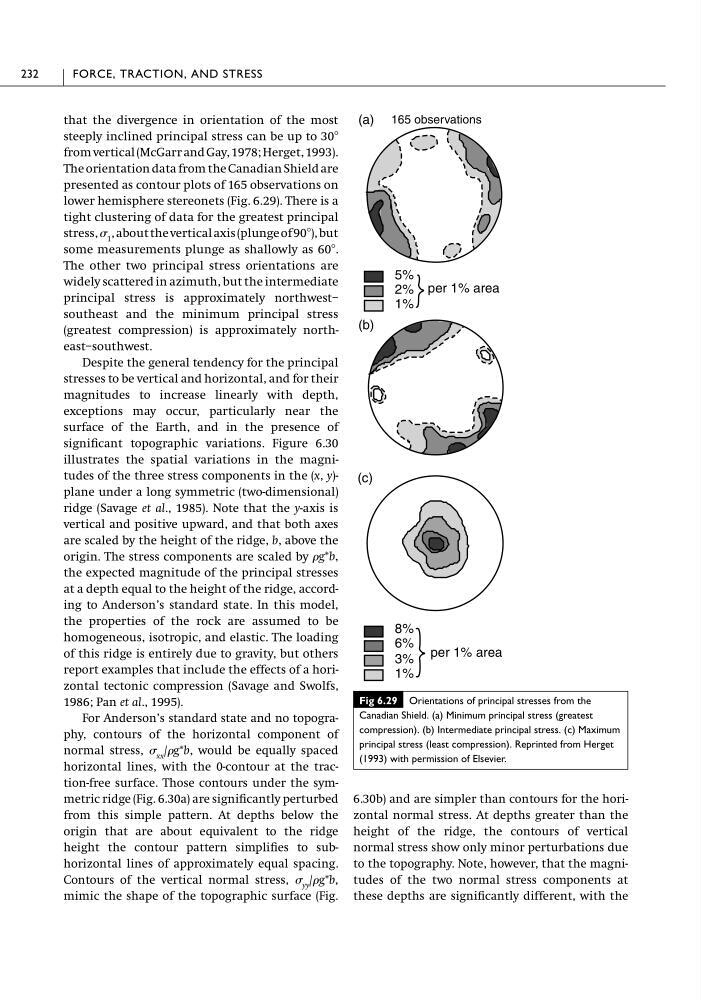
The orientation data from the Canadian Shield are
presented as contour plots of 165 observations on
lower hemisphere stereonets (Fig. 6.29). There is a
tight clustering of data for the greatest principal
stress, 1 , about the vertical axis (plunge of 90Њ), but
some measurements plunge as shallowly as 60Њ.
The other two principal stress orientations are
widely scattered in azimuth, but the intermediate
principal stress is approximately northwest–
southeast and the minimum principal stress
(greatest compression) is approximately northeast–southwest.
Despite the general tendency for the principal
stresses to be vertical and horizontal, and for their
magnitudes to increase linearly with depth,
exceptions may occur, particularly near the
surface of the Earth, and in the presence of
significant topographic variations. Figure 6.30
illustrates the spatial variations in the magnitudes of the three stress components in the (x, y)plane under a long symmetric (two-dimensional)
ridge (Savage et al., 1985). Note that the y-axis is
vertical and positive upward, and that both axes
are scaled by the height of the ridge, b, above the
origin. The stress components are scaled by g*b,
the expected magnitude of the principal stresses
at a depth equal to the height of the ridge, according to Anderson’s standard state. In this model,
the properties of the rock are assumed to be
homogeneous, isotropic, and elastic. The loading
of this ridge is entirely due to gravity, but others
report examples that include the effects of a horizontal tectonic compression (Savage and Swolfs,
1986; Pan et al., 1995).
For Anderson’s standard state and no topography, contours of the horizontal component of
normal stress, xx /g*b, would be equally spaced
horizontal lines, with the 0-contour at the traction-free surface. Those contours under the symmetric ridge (Fig. 6.30a) are significantly perturbed
from this simple pattern. At depths below the
origin that are about equivalent to the ridge
height the contour pattern simplifies to subhorizontal lines of approximately equal spacing.
Contours of the vertical normal stress, yy /g*b,
mimic the shape of the topographic surface (Fig.
6.30b) and are simpler than contours for the horizontal normal stress. At depths greater than the
height of the ridge, the contours of vertical
normal stress show only minor perturbations due
to the topography. Note, however, that the magnitudes of the two normal stress components at
these depths are significantly different, with the
232
FORCE, TRACTION, AND STRESS
Fig 6.29 Orientations of principal stresses from the
Canadian Shield. (a) Minimum principal stress (greatest
compression). (b) Intermediate principal stress. (c) Maximum
principal stress (least compression). Reprinted from Herget
(1993) with permission of Elsevier.
1%
5%
2%
3%
8%
6%
1%
per 1% area
165 observations
per 1% area
(a)
(b)
(c)
steeply inclined principal stress can be up to 30Њ
from vertical (McGarr and Gay, 1978; Herget, 1993).
The orientation data from the Canadian Shield are
presented as contour plots of 165 observations on
lower hemisphere stereonets (Fig. 6.29). There is a
tight clustering of data for the greatest principal
stress, 1 , about the vertical axis (plunge of 90Њ), but
some measurements plunge as shallowly as 60Њ.
The other two principal stress orientations are
widely scattered in azimuth, but the intermediate
principal stress is approximately northwest–
southeast and the minimum principal stress
(greatest compression) is approximately northeast–southwest.
Despite the general tendency for the principal
stresses to be vertical and horizontal, and for their
magnitudes to increase linearly with depth,
exceptions may occur, particularly near the
surface of the Earth, and in the presence of
significant topographic variations. Figure 6.30
illustrates the spatial variations in the magnitudes of the three stress components in the (x, y)plane under a long symmetric (two-dimensional)
ridge (Savage et al., 1985). Note that the y-axis is
vertical and positive upward, and that both axes
are scaled by the height of the ridge, b, above the
origin. The stress components are scaled by g*b,
the expected magnitude of the principal stresses
at a depth equal to the height of the ridge, according to Anderson’s standard state. In this model,
the properties of the rock are assumed to be
homogeneous, isotropic, and elastic. The loading
of this ridge is entirely due to gravity, but others
report examples that include the effects of a horizontal tectonic compression (Savage and Swolfs,
1986; Pan et al., 1995).
For Anderson’s standard state and no topography, contours of the horizontal component of
normal stress, xx /g*b, would be equally spaced
horizontal lines, with the 0-contour at the traction-free surface. Those contours under the symmetric ridge (Fig. 6.30a) are significantly perturbed
from this simple pattern. At depths below the
origin that are about equivalent to the ridge
height the contour pattern simplifies to subhorizontal lines of approximately equal spacing.
Contours of the vertical normal stress, yy /g*b,
mimic the shape of the topographic surface (Fig.
6.30b) and are simpler than contours for the horizontal normal stress. At depths greater than the
height of the ridge, the contours of vertical
normal stress show only minor perturbations due
to the topography. Note, however, that the magnitudes of the two normal stress components at
these depths are significantly different, with the
232
FORCE, TRACTION, AND STRESS
Fig 6.29 Orientations of principal stresses from the
Canadian Shield. (a) Minimum principal stress (greatest
compression). (b) Intermediate principal stress. (c) Maximum
principal stress (least compression). Reprinted from Herget
(1993) with permission of Elsevier.
1%
5%
2%
3%
8%
6%
1%
per 1% area
165 observations
per 1% area
(a)
(b)
(c)