

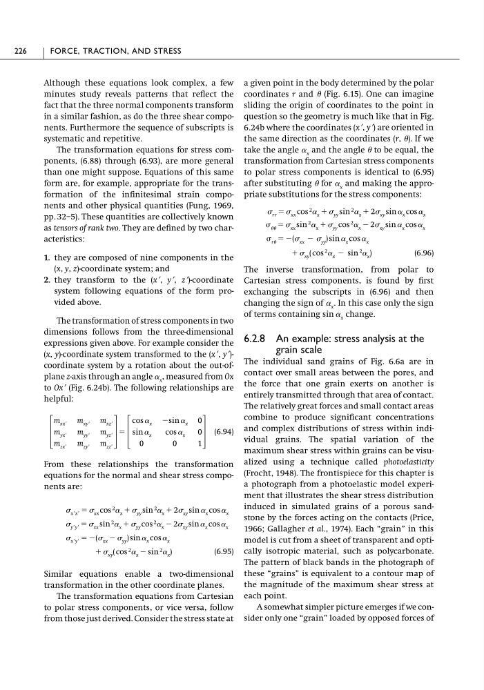
Although these equations look complex, a few
minutes study reveals patterns that reflect the
fact that the three normal components transform
in a similar fashion, as do the three shear components. Furthermore the sequence of subscripts is
systematic and repetitive.
The transformation equations for stress components, (6.88) through (6.93), are more general
than one might suppose. Equations of this same
form are, for example, appropriate for the transformation of the infinitesimal strain components and other physical quantities (Fung, 1969,
pp. 32–5). These quantities are collectively known
as tensors of rank two. They are defined by two characteristics:
1. they are composed of nine components in the
(x, y, z)-coordinate system; and
2. they transform to the (xЈ, yЈ, zЈ)-coordinate
system following equations of the form provided above.
The transformation of stress components in two
dimensions follows from the three-dimensional
expressions given above. For example consider the
(x, y)-coordinate system transformed to the (xЈ, yЈ)coordinate system by a rotation about the out-ofplane z-axis through an angle ␣ x , measured from Ox
to OxЈ (Fig. 6.24b). The following relationships are
helpful:
(6.94)
From these relationships the transformation
equations for the normal and shear stress components are:
(6.95)
Similar equations enable a two-dimensional
transformation in the other coordinate planes.
The transformation equations from Cartesian
to polar stress components, or vice versa, follow
from those just derived. Consider the stress state at
ϩ xy ( cos 2 ␣ x Ϫ sin 2 ␣ x )
xЈyЈ ϭ Ϫ( xx Ϫ yy ) sin ␣ x cos ␣ x
yЈyЈ ϭ xx sin 2 ␣ x ϩ yy cos 2 ␣ x Ϫ 2 xy sin ␣ x cos ␣ x
xЈxЈ ϭ xx cos 2 ␣ x ϩ yy sin 2 ␣ x ϩ 2 xy sin ␣ x cos ␣ x
΄
m xxЈ m xyЈ m xzЈ
m yxЈ m yyЈ m yzЈ
m zxЈ m zyЈ m zzЈ
΅
ϭ
΄
cos ␣ x Ϫsin ␣ x 0
sin ␣ x
cos ␣ x 0
0
0
1
΅
a given point in the body determined by the polar
coordinates r and (Fig. 6.15). One can imagine
sliding the origin of coordinates to the point in
question so the geometry is much like that in Fig.
6.24b where the coordinates (xЈ, yЈ) are oriented in
the same direction as the coordinates (r, ). If we
take the angle ␣ x and the angle to be equal, the
transformation from Cartesian stress components
to polar stress components is identical to (6.95)
after substituting for ␣ x and making the appropriate substitutions for the stress components:
(6.96)
The inverse transformation, from polar to
Cartesian stress components, is found by first
exchanging the subscripts in (6.96) and then
changing the sign of ␣ x . In this case only the sign
of terms containing sin ␣ x change.
6.2.8 An example: stress analysis at the
grain scale
The individual sand grains of Fig. 6.6a are in
contact over small areas between the pores, and
the force that one grain exerts on another is
entirely transmitted through that area of contact.
The relatively great forces and small contact areas
combine to produce significant concentrations
and complex distributions of stress within individual grains. The spatial variation of the
maximum shear stress within grains can be visualized using a technique called photoelasticity
(Frocht, 1948). The frontispiece for this chapter is
a photograph from a photoelastic model experiment that illustrates the shear stress distribution
induced in simulated grains of a porous sandstone by the forces acting on the contacts (Price,
1966; Gallagher et al., 1974). Each “grain” in this
model is cut from a sheet of transparent and optically isotropic material, such as polycarbonate.
The pattern of black bands in the photograph of
these “grains” is equivalent to a contour map of
the magnitude of the maximum shear stress at
each point.
A somewhat simpler picture emerges if we consider only one “grain” loaded by opposed forces of
ϩ xy ( cos
2 ␣ x Ϫ sin
2
␣ x )
r ϭ Ϫ( xx Ϫ yy ) sin ␣ x cos ␣ x
ϭ xx sin
2 ␣ x ϩ yy cos
2 ␣ x Ϫ 2 xy sin ␣ x cos ␣ x
rr ϭ xx cos 2 ␣ x ϩ yy sin 2 ␣ x ϩ 2 xy sin ␣ x cos ␣ x
226
FORCE, TRACTION, AND STRESS
minutes study reveals patterns that reflect the
fact that the three normal components transform
in a similar fashion, as do the three shear components. Furthermore the sequence of subscripts is
systematic and repetitive.
The transformation equations for stress components, (6.88) through (6.93), are more general
than one might suppose. Equations of this same
form are, for example, appropriate for the transformation of the infinitesimal strain components and other physical quantities (Fung, 1969,
pp. 32–5). These quantities are collectively known
as tensors of rank two. They are defined by two characteristics:
1. they are composed of nine components in the
(x, y, z)-coordinate system; and
2. they transform to the (xЈ, yЈ, zЈ)-coordinate
system following equations of the form provided above.
The transformation of stress components in two
dimensions follows from the three-dimensional
expressions given above. For example consider the
(x, y)-coordinate system transformed to the (xЈ, yЈ)coordinate system by a rotation about the out-ofplane z-axis through an angle ␣ x , measured from Ox
to OxЈ (Fig. 6.24b). The following relationships are
helpful:
(6.94)
From these relationships the transformation
equations for the normal and shear stress components are:
(6.95)
Similar equations enable a two-dimensional
transformation in the other coordinate planes.
The transformation equations from Cartesian
to polar stress components, or vice versa, follow
from those just derived. Consider the stress state at
ϩ xy ( cos 2 ␣ x Ϫ sin 2 ␣ x )
xЈyЈ ϭ Ϫ( xx Ϫ yy ) sin ␣ x cos ␣ x
yЈyЈ ϭ xx sin 2 ␣ x ϩ yy cos 2 ␣ x Ϫ 2 xy sin ␣ x cos ␣ x
xЈxЈ ϭ xx cos 2 ␣ x ϩ yy sin 2 ␣ x ϩ 2 xy sin ␣ x cos ␣ x
΄
m xxЈ m xyЈ m xzЈ
m yxЈ m yyЈ m yzЈ
m zxЈ m zyЈ m zzЈ
΅
ϭ
΄
cos ␣ x Ϫsin ␣ x 0
sin ␣ x
cos ␣ x 0
0
0
1
΅
a given point in the body determined by the polar
coordinates r and (Fig. 6.15). One can imagine
sliding the origin of coordinates to the point in
question so the geometry is much like that in Fig.
6.24b where the coordinates (xЈ, yЈ) are oriented in
the same direction as the coordinates (r, ). If we
take the angle ␣ x and the angle to be equal, the
transformation from Cartesian stress components
to polar stress components is identical to (6.95)
after substituting for ␣ x and making the appropriate substitutions for the stress components:
(6.96)
The inverse transformation, from polar to
Cartesian stress components, is found by first
exchanging the subscripts in (6.96) and then
changing the sign of ␣ x . In this case only the sign
of terms containing sin ␣ x change.
6.2.8 An example: stress analysis at the
grain scale
The individual sand grains of Fig. 6.6a are in
contact over small areas between the pores, and
the force that one grain exerts on another is
entirely transmitted through that area of contact.
The relatively great forces and small contact areas
combine to produce significant concentrations
and complex distributions of stress within individual grains. The spatial variation of the
maximum shear stress within grains can be visualized using a technique called photoelasticity
(Frocht, 1948). The frontispiece for this chapter is
a photograph from a photoelastic model experiment that illustrates the shear stress distribution
induced in simulated grains of a porous sandstone by the forces acting on the contacts (Price,
1966; Gallagher et al., 1974). Each “grain” in this
model is cut from a sheet of transparent and optically isotropic material, such as polycarbonate.
The pattern of black bands in the photograph of
these “grains” is equivalent to a contour map of
the magnitude of the maximum shear stress at
each point.
A somewhat simpler picture emerges if we consider only one “grain” loaded by opposed forces of
ϩ xy ( cos
2 ␣ x Ϫ sin
2
␣ x )
r ϭ Ϫ( xx Ϫ yy ) sin ␣ x cos ␣ x
ϭ xx sin
2 ␣ x ϩ yy cos
2 ␣ x Ϫ 2 xy sin ␣ x cos ␣ x
rr ϭ xx cos 2 ␣ x ϩ yy sin 2 ␣ x ϩ 2 xy sin ␣ x cos ␣ x
226
FORCE, TRACTION, AND STRESS