

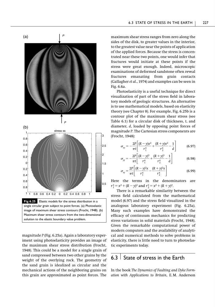
magnitude P (Fig. 6.25a). Again a laboratory experiment using photoelasticity provides an image of
the maximum shear stress distribution (Frocht,
1948). This could be a model for a single grain of
sand compressed between two other grains by the
weight of the overlying rock. The geometry of
the sand grain is idealized as circular and the
mechanical actions of the neighboring grains on
this grain are approximated as point forces. The
maximum shear stress ranges from zero along the
sides of the disk, to greater values in the interior,
to the greatest value near the points of application
of the applied forces. Because the stress is concentrated near these two points, one would infer that
fractures would initiate at these points if the
stress were great enough. Indeed, microscopic
examinations of deformed sandstone often reveal
fractures emanating from grain contacts
(Gallagher et al., 1974) and examples can be seen in
Fig. 6.6a.
Photoelasticity is a useful technique for direct
visualization of part of the stress field in laboratory models of geologic structures. An alternative
is to use mathematical models, based on elasticity
theory (see Chapter 8). For example, Fig. 6.25b is a
contour plot of the maximum shear stress (see
Table 6.1) for a circular disk of thickness, t, and
diameter, d, loaded by opposing point forces of
magnitude P. The Cartesian stress components are
(Frocht, 1948):
(6.97)
(6.98)
(6.99)
Here the terms in the denominators are
.
There is a remarkable similarity between the
stress field calculated from the mathematical
model (6.97) and the stress field visualized in the
analogous laboratory experiment (Fig. 6.25a).
Many such examples have demonstrated the
efficacy of continuum mechanics for predicting
stress variations in solid materials (Frocht, 1948).
Given the remarkable computational power of
modern computers and the availability of analytical and numerical methods to solve problems in
elasticity, there is little need to turn to photoelastic experiments today.
6.3 State of stress in the Earth
In the book The Dynamics of Faulting and Dyke Formation with Applications to Britain, E. M. Anderson
r 2
1 ϭ x 2 ϩ (R Ϫ y) 2 and r 2
2 ϭ x 2 ϩ (R ϩ y) 2
xy ϭ
2P
t ΄
(R Ϫ y) 2 x
r 4
1
Ϫ
(R ϩ y) 2 x
r 4
2
΅
yy ϭ Ϫ
2P
t ΄
(R Ϫ y) 3
r 4
1
ϩ
(R ϩ y) 3
r 4
2
Ϫ
1
d ΅
xx ϭ Ϫ
2P
t ΄
(R Ϫ y)x 2
r 4
1
ϩ
(R ϩ y)x 2
r 4
2
Ϫ
1
d ΅
6.3 STATE OF STRESS IN THE EARTH
227
Fig 6.25 Elastic models for the stress distribution in a
single circular grain subject to point forces. (a) Photoelastic
image of maximum shear stress contours (Frocht, 1948). (b)
Maximum shear stress contours from the two-dimensional
solution to the elastic boundary value problem.
(a)
(b)
stress ss
P
P
1
0.8
0.6
0.4
0.2
0
0.2
0.4
0.6
0.8
1 1 0.8 0.6 0.4 0.2 0 0.2 0.4 0.6 0.8 1
3
2.5
2
1.5
1
0.5
the maximum shear stress distribution (Frocht,
1948). This could be a model for a single grain of
sand compressed between two other grains by the
weight of the overlying rock. The geometry of
the sand grain is idealized as circular and the
mechanical actions of the neighboring grains on
this grain are approximated as point forces. The
maximum shear stress ranges from zero along the
sides of the disk, to greater values in the interior,
to the greatest value near the points of application
of the applied forces. Because the stress is concentrated near these two points, one would infer that
fractures would initiate at these points if the
stress were great enough. Indeed, microscopic
examinations of deformed sandstone often reveal
fractures emanating from grain contacts
(Gallagher et al., 1974) and examples can be seen in
Fig. 6.6a.
Photoelasticity is a useful technique for direct
visualization of part of the stress field in laboratory models of geologic structures. An alternative
is to use mathematical models, based on elasticity
theory (see Chapter 8). For example, Fig. 6.25b is a
contour plot of the maximum shear stress (see
Table 6.1) for a circular disk of thickness, t, and
diameter, d, loaded by opposing point forces of
magnitude P. The Cartesian stress components are
(Frocht, 1948):
(6.97)
(6.98)
(6.99)
Here the terms in the denominators are
.
There is a remarkable similarity between the
stress field calculated from the mathematical
model (6.97) and the stress field visualized in the
analogous laboratory experiment (Fig. 6.25a).
Many such examples have demonstrated the
efficacy of continuum mechanics for predicting
stress variations in solid materials (Frocht, 1948).
Given the remarkable computational power of
modern computers and the availability of analytical and numerical methods to solve problems in
elasticity, there is little need to turn to photoelastic experiments today.
6.3 State of stress in the Earth
In the book The Dynamics of Faulting and Dyke Formation with Applications to Britain, E. M. Anderson
r 2
1 ϭ x 2 ϩ (R Ϫ y) 2 and r 2
2 ϭ x 2 ϩ (R ϩ y) 2
xy ϭ
2P
t ΄
(R Ϫ y) 2 x
r 4
1
Ϫ
(R ϩ y) 2 x
r 4
2
΅
yy ϭ Ϫ
2P
t ΄
(R Ϫ y) 3
r 4
1
ϩ
(R ϩ y) 3
r 4
2
Ϫ
1
d ΅
xx ϭ Ϫ
2P
t ΄
(R Ϫ y)x 2
r 4
1
ϩ
(R ϩ y)x 2
r 4
2
Ϫ
1
d ΅
6.3 STATE OF STRESS IN THE EARTH
227
Fig 6.25 Elastic models for the stress distribution in a
single circular grain subject to point forces. (a) Photoelastic
image of maximum shear stress contours (Frocht, 1948). (b)
Maximum shear stress contours from the two-dimensional
solution to the elastic boundary value problem.
(a)
(b)
stress ss
P
P
1
0.8
0.6
0.4
0.2
0
0.2
0.4
0.6
0.8
1 1 0.8 0.6 0.4 0.2 0 0.2 0.4 0.6 0.8 1
3
2.5
2
1.5
1
0.5