

stresses. The circle with a center at AЈ traces out
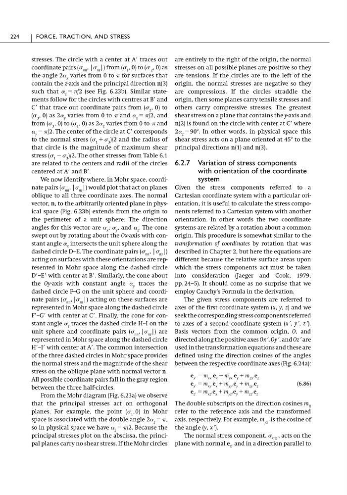
coordinate pairs ( nn , | ns |) from ( 1 , 0) to ( 2 , 0) as
the angle 2␣ x varies from 0 to for surfaces that
contain the z-axis and the principal direction n(3)
such that ␣ z ϭ /2 (see Fig. 6.23b). Similar statements follow for the circles with centres at BЈ and
CЈ that trace out coordinate pairs from ( 2 , 0) to
( 3 , 0) as 2␣ y varies from 0 to and ␣ x ϭ /2, and
from ( 3 , 0) to ( 1 , 0) as 2␣ z varies from 0 to and
␣ y ϭ /2. The center of the circle at CЈ corresponds
to the normal stress ( 1 ϩ 3 )/2 and the radius of
that circle is the magnitude of maximum shear
stress ( 1 Ϫ 3 )/2. The other stresses from Table 6.1
are related to the centers and radii of the circles
centered at AЈ and BЈ.
We now identify where, in Mohr space, coordinate pairs ( nn , | ns |) would plot that act on planes
oblique to all three coordinate axes. The normal
vector, n, to the arbitrarily oriented plane in physical space (Fig. 6.23b) extends from the origin to
the perimeter of a unit sphere. The direction
angles for this vector are ␣ x , ␣ y , and ␣ z . The cone
swept out by rotating about the Ox-axis with constant angle ␣ x intersects the unit sphere along the
dashed circle D–E. The coordinate pairs ( nn , | ns |)
acting on surfaces with these orientations are represented in Mohr space along the dashed circle
DЈ–EЈ with center at BЈ. Similarly, the cone about
the Oy-axis with constant angle ␣ y traces the
dashed circle F–G on the unit sphere and coordinate pairs ( nn ,| ns |) acting on these surfaces are
represented in Mohr space along the dashed circle
FЈ–GЈ with center at CЈ. Finally, the cone for constant angle ␣ z traces the dashed circle H–I on the
unit sphere and coordinate pairs ( nn ,| ns |) are
represented in Mohr space along the dashed circle
HЈ–IЈ with center at AЈ. The common intersection
of the three dashed circles in Mohr space provides
the normal stress and the magnitude of the shear
stress on the oblique plane with normal vector n.
All possible coordinate pairs fall in the gray region
between the three half-circles.
From the Mohr diagram (Fig. 6.23a) we observe
that the principal stresses act on orthogonal
planes. For example, the point ( 1 , 0) in Mohr
space is associated with the double angle 2␣ z ϭ ,
so in physical space we have ␣ z ϭ /2. Because the
principal stresses plot on the abscissa, the principal planes carry no shear stress. If the Mohr circles
are entirely to the right of the origin, the normal
stresses on all possible planes are positive so they
are tensions. If the circles are to the left of the
origin, the normal stresses are negative so they
are compressions. If the circles straddle the
origin, then some planes carry tensile stresses and
others carry compressive stresses. The greatest
shear stress on a plane that contains the y-axis and
n(2) is found on the circle with center at CЈ where
2␣ z ϭ 90Њ. In other words, in physical space this
shear stress acts on a plane oriented at 45Њ to the
principal directions n(1) and n(3).
6.2.7 Variation of stress components
with orientation of the coordinate
system
Given the stress components referred to a
Cartesian coordinate system with a particular orientation, it is useful to calculate the stress components referred to a Cartesian system with another
orientation. In other words the two coordinate
systems are related by a rotation about a common
origin. This procedure is somewhat similar to the
transformation of coordinates by rotation that was
described in Chapter 2, but here the equations are
different because the relative surface areas upon
which the stress components act must be taken
into consideration (Jaeger and Cook, 1979,
pp. 24–5). It should come as no surprise that we
employ Cauchy’s Formula in the derivation.
The given stress components are referred to
axes of the first coordinate system (x, y, z) and we
seek the corresponding stress components referred
to axes of a second coordinate system (xЈ, yЈ, zЈ).
Basis vectors from the common origin, O, and
directed along the positive axes OxЈ, OyЈ, and OzЈ are
used in the transformation equations and these are
defined using the direction cosines of the angles
between the respective coordinate axes (Fig. 6.24a):
(6.86)
The double subscripts on the direction cosines m ij
refer to the reference axis and the transformed
axis, respectively. For example, m yxЈ is the cosine of
the angle (y, xЈ).
The normal stress component, xЈxЈ , acts on the
plane with normal e xЈ and in a direction parallel to
e zЈ ϭ m xzЈ e x ϩ m yzЈ e y ϩ m zzЈ e z
e yЈ ϭ m xyЈ e x ϩ m yyЈ e y ϩ m zyЈ e z
e xЈ ϭ m xxЈ e x ϩ m yxЈ e y ϩ m zxЈ e z
224
FORCE, TRACTION, AND STRESS
coordinate pairs ( nn , | ns |) from ( 1 , 0) to ( 2 , 0) as
the angle 2␣ x varies from 0 to for surfaces that
contain the z-axis and the principal direction n(3)
such that ␣ z ϭ /2 (see Fig. 6.23b). Similar statements follow for the circles with centres at BЈ and
CЈ that trace out coordinate pairs from ( 2 , 0) to
( 3 , 0) as 2␣ y varies from 0 to and ␣ x ϭ /2, and
from ( 3 , 0) to ( 1 , 0) as 2␣ z varies from 0 to and
␣ y ϭ /2. The center of the circle at CЈ corresponds
to the normal stress ( 1 ϩ 3 )/2 and the radius of
that circle is the magnitude of maximum shear
stress ( 1 Ϫ 3 )/2. The other stresses from Table 6.1
are related to the centers and radii of the circles
centered at AЈ and BЈ.
We now identify where, in Mohr space, coordinate pairs ( nn , | ns |) would plot that act on planes
oblique to all three coordinate axes. The normal
vector, n, to the arbitrarily oriented plane in physical space (Fig. 6.23b) extends from the origin to
the perimeter of a unit sphere. The direction
angles for this vector are ␣ x , ␣ y , and ␣ z . The cone
swept out by rotating about the Ox-axis with constant angle ␣ x intersects the unit sphere along the
dashed circle D–E. The coordinate pairs ( nn , | ns |)
acting on surfaces with these orientations are represented in Mohr space along the dashed circle
DЈ–EЈ with center at BЈ. Similarly, the cone about
the Oy-axis with constant angle ␣ y traces the
dashed circle F–G on the unit sphere and coordinate pairs ( nn ,| ns |) acting on these surfaces are
represented in Mohr space along the dashed circle
FЈ–GЈ with center at CЈ. Finally, the cone for constant angle ␣ z traces the dashed circle H–I on the
unit sphere and coordinate pairs ( nn ,| ns |) are
represented in Mohr space along the dashed circle
HЈ–IЈ with center at AЈ. The common intersection
of the three dashed circles in Mohr space provides
the normal stress and the magnitude of the shear
stress on the oblique plane with normal vector n.
All possible coordinate pairs fall in the gray region
between the three half-circles.
From the Mohr diagram (Fig. 6.23a) we observe
that the principal stresses act on orthogonal
planes. For example, the point ( 1 , 0) in Mohr
space is associated with the double angle 2␣ z ϭ ,
so in physical space we have ␣ z ϭ /2. Because the
principal stresses plot on the abscissa, the principal planes carry no shear stress. If the Mohr circles
are entirely to the right of the origin, the normal
stresses on all possible planes are positive so they
are tensions. If the circles are to the left of the
origin, the normal stresses are negative so they
are compressions. If the circles straddle the
origin, then some planes carry tensile stresses and
others carry compressive stresses. The greatest
shear stress on a plane that contains the y-axis and
n(2) is found on the circle with center at CЈ where
2␣ z ϭ 90Њ. In other words, in physical space this
shear stress acts on a plane oriented at 45Њ to the
principal directions n(1) and n(3).
6.2.7 Variation of stress components
with orientation of the coordinate
system
Given the stress components referred to a
Cartesian coordinate system with a particular orientation, it is useful to calculate the stress components referred to a Cartesian system with another
orientation. In other words the two coordinate
systems are related by a rotation about a common
origin. This procedure is somewhat similar to the
transformation of coordinates by rotation that was
described in Chapter 2, but here the equations are
different because the relative surface areas upon
which the stress components act must be taken
into consideration (Jaeger and Cook, 1979,
pp. 24–5). It should come as no surprise that we
employ Cauchy’s Formula in the derivation.
The given stress components are referred to
axes of the first coordinate system (x, y, z) and we
seek the corresponding stress components referred
to axes of a second coordinate system (xЈ, yЈ, zЈ).
Basis vectors from the common origin, O, and
directed along the positive axes OxЈ, OyЈ, and OzЈ are
used in the transformation equations and these are
defined using the direction cosines of the angles
between the respective coordinate axes (Fig. 6.24a):
(6.86)
The double subscripts on the direction cosines m ij
refer to the reference axis and the transformed
axis, respectively. For example, m yxЈ is the cosine of
the angle (y, xЈ).
The normal stress component, xЈxЈ , acts on the
plane with normal e xЈ and in a direction parallel to
e zЈ ϭ m xzЈ e x ϩ m yzЈ e y ϩ m zzЈ e z
e yЈ ϭ m xyЈ e x ϩ m yyЈ e y ϩ m zyЈ e z
e xЈ ϭ m xxЈ e x ϩ m yxЈ e y ϩ m zxЈ e z
224
FORCE, TRACTION, AND STRESS