

act on planes that contain one of the principal
normal stress directions and bisect the angle
between the other two, so the normals to these
planes make angles of Ϯ45
o with the principal axes
of normal stress (Fig. 6.22). The magnitudes of the
maximum shear stresses are one-half of the difference between the associated principal normal
stresses. Recall that the principal normal stresses
act on planes that carry zero shear stress. In contrast, the maximum shear stresses act on planes
that have a normal stress equal in magnitude to the
average of the associated principal normal stresses.
6.2.6 The Mohr diagram: visualizing
stress variation for a given stress
state
The variation of normal and shear stress with the
orientation of the boundary on which they act in a
region of homogeneous stress can be appreciated
using a graphical construction called the Mohr
diagram. Apparently the German civil engineer
Otto Mohr first described this graphical construction in 1882 (Mohr, 1882; Timoshenko and Goodier,
1970). Since then it has been used in countless textbooks and journal articles, becoming a standard
tool for stress analysis. The need for graphical constructions for the analysis of stress variation has
largely been made obsolete by computers. The technique is reviewed here for historical reasons and
to reinforce the intuitive understanding of these
variations.
Detailed derivations of the equations behind
the Mohr diagram are provided elsewhere
(Malvern, 1969; Jaeger and Cook, 1979), so we only
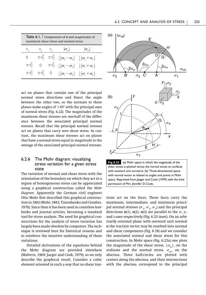
describe the graphical result. Consider a cubic
element oriented in such a way that no shear tractions act on the faces. These faces carry the
maximum, intermediate, and minimum principal normal stresses ( 1 , 2 , 3 ) and the principal
directions n(1), n(2), n(3) are parallel to the x-, y-,
and z-axes respectively (Fig. 6.23 inset). On an arbitrarily oriented plane with outward unit normal
n the traction vector may be resolved into normal
and shear components (Fig. 6.18) and we consider
the associated normal and shear stress for this
construction. In Mohr space (Fig. 6.23a) one plots
the magnitude of the shear stress, | ns |, on the
ordinate and the normal stress, nn , on the
abscissa. Three half-circles are plotted with
centers along the abscissa, and their intersections
with the abscissa correspond to the principal
6.2 CONCEPT AND ANALYSIS OF STRESS
223
Table 6.1. Components of n and magnitudes of
maximum shear stress and normal stress.
n x
n y
n z
| ns |
| nn |
0
0
0
1
2 | 1 ϩ 2 |
1
2 | 1 Ϫ 2 |
Ϯ√
1
2
Ϯ√
1
2
1
2 | 1 ϩ 3 |
1
2 | 1 Ϫ 3 |
Ϯ√
1
2
Ϯ√
1
2
1
2 | 2 ϩ 3 |
1
2 | 2 Ϫ 3 |
Ϯ√
1
2
Ϯ√
1
2
Fig 6.23 (a) Mohr space in which the magnitude of the
shear stress is plotted versus the normal stress on surfaces
with outward unit normal n. (b) Three-dimensional space
with normal vector n related to angles and points in Mohr
space. Reprinted from Jaeger and Cook (1979) with the kind
permission of Mrs. Jennifer D. Cook.
|s ns |
x
y
z
a x
n
G
H
I
E
AЈ
BЈ
CЈ
DЈ
EЈ
GЈ
HЈ
(a)
(b)
a z
2a y
2a x
s nn
s 1
s 2
s 3
a y
x
y
z
s 2
s 3
s 1
2a z
F
D
FЈ
IЈ
normal stress directions and bisect the angle
between the other two, so the normals to these
planes make angles of Ϯ45
o with the principal axes
of normal stress (Fig. 6.22). The magnitudes of the
maximum shear stresses are one-half of the difference between the associated principal normal
stresses. Recall that the principal normal stresses
act on planes that carry zero shear stress. In contrast, the maximum shear stresses act on planes
that have a normal stress equal in magnitude to the
average of the associated principal normal stresses.
6.2.6 The Mohr diagram: visualizing
stress variation for a given stress
state
The variation of normal and shear stress with the
orientation of the boundary on which they act in a
region of homogeneous stress can be appreciated
using a graphical construction called the Mohr
diagram. Apparently the German civil engineer
Otto Mohr first described this graphical construction in 1882 (Mohr, 1882; Timoshenko and Goodier,
1970). Since then it has been used in countless textbooks and journal articles, becoming a standard
tool for stress analysis. The need for graphical constructions for the analysis of stress variation has
largely been made obsolete by computers. The technique is reviewed here for historical reasons and
to reinforce the intuitive understanding of these
variations.
Detailed derivations of the equations behind
the Mohr diagram are provided elsewhere
(Malvern, 1969; Jaeger and Cook, 1979), so we only
describe the graphical result. Consider a cubic
element oriented in such a way that no shear tractions act on the faces. These faces carry the
maximum, intermediate, and minimum principal normal stresses ( 1 , 2 , 3 ) and the principal
directions n(1), n(2), n(3) are parallel to the x-, y-,
and z-axes respectively (Fig. 6.23 inset). On an arbitrarily oriented plane with outward unit normal
n the traction vector may be resolved into normal
and shear components (Fig. 6.18) and we consider
the associated normal and shear stress for this
construction. In Mohr space (Fig. 6.23a) one plots
the magnitude of the shear stress, | ns |, on the
ordinate and the normal stress, nn , on the
abscissa. Three half-circles are plotted with
centers along the abscissa, and their intersections
with the abscissa correspond to the principal
6.2 CONCEPT AND ANALYSIS OF STRESS
223
Table 6.1. Components of n and magnitudes of
maximum shear stress and normal stress.
n x
n y
n z
| ns |
| nn |
0
0
0
1
2 | 1 ϩ 2 |
1
2 | 1 Ϫ 2 |
Ϯ√
1
2
Ϯ√
1
2
1
2 | 1 ϩ 3 |
1
2 | 1 Ϫ 3 |
Ϯ√
1
2
Ϯ√
1
2
1
2 | 2 ϩ 3 |
1
2 | 2 Ϫ 3 |
Ϯ√
1
2
Ϯ√
1
2
Fig 6.23 (a) Mohr space in which the magnitude of the
shear stress is plotted versus the normal stress on surfaces
with outward unit normal n. (b) Three-dimensional space
with normal vector n related to angles and points in Mohr
space. Reprinted from Jaeger and Cook (1979) with the kind
permission of Mrs. Jennifer D. Cook.
|s ns |
x
y
z
a x
n
G
H
I
E
AЈ
BЈ
CЈ
DЈ
EЈ
GЈ
HЈ
(a)
(b)
a z
2a y
2a x
s nn
s 1
s 2
s 3
a y
x
y
z
s 2
s 3
s 1
2a z
F
D
FЈ
IЈ