

principal stress, 3 (maximum compressive
stress). The triangulated surfaces are model fault
surfaces for a hydrocarbon reservoir in the North
Sea and the principal stresses were used to predict
the location and orientation of small faults in this
reservoir (Maerten et al., 2002).
The orientation of the Cartesian coordinate
system in the preceding discussion of principal
stresses was arbitrary. Any orientation could be
chosen and the resulting principal stresses and
principal axes would be identical. In other words
the three roots of the cubic equation (6.59) are the
same, regardless of coordinate system, so the
coefficients of this equation must not vary for a
given state of stress. Rewriting this cubic equation
by collecting the stress components into constant
coefficients we have:
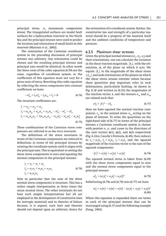
(6.74)
The invariant coefficients are:
(6.75)
These combinations of the Cartesian stress components are referred to as the stress invariants.
The definitions of the stress invariants in
terms of the Cartesian components are reduced to
definitions in terms of the principal stresses by
rotating the coordinate system until it aligns with
the principal axes. This is equivalent to setting the
shear stress components to zero and equating the
normal components to the principal stresses:
(6.76)
Note in particular that the sum of the three
normal stress components is invariant. This has a
rather simple interpretation as three times the
mean normal stress. The other invariants do not
have such simple interpretations but all are
employed in the development of constitutive laws
for isotropic materials and in theories of failure
because, it is argued, such laws and theories
should not depend upon an arbitrary choice for
I 3 ϭ 1 2 3
I 2 ϭ 1 2 ϩ 2 3 ϩ 3 2
I 1 ϭ 1 ϩ 2 ϩ 3
I 3 ϭ xx yy zz ϩ 2 xy yz zx Ϫ xx 2
yz Ϫ yy 2
zx Ϫ zz 2
xy
I 2 ϭ xx yy ϩ yy zz ϩ zz xx Ϫ
2
xy
Ϫ
2
yz
Ϫ
2
zx
I 1 ϭ xx ϩ yy ϩ zz
Ϫ 3
nn ϩ I 1 2
nn Ϫ I 2 nn ϩ I 3 ϭ 0
the orientation of a coordinate system. Rather, the
constitutive law and strength of a particular material should be a property of the material itself
and the ambient conditions of temperature and
pressure.
6.2.5 Maximum shear stresses
Given the principal normal stresses ( 1 , 2 , 3 ) and
their orientations, one can calculate the variation
in the shear traction magnitude, |t s |, with the orientation, n, of the plane on which it acts. We
equate |t s | to the magnitude of the shear stress
| ns | and seek orientations of the planes on which
the shear stress attains extreme values because
these quantities play important roles in rock
deformation, particularly faulting. As shown in
Fig. 6.18 and written in (6.53) the magnitudes of
the traction vector, t, and the stresses ns and nn
are related such that:
(6.77)
Here we have equated the normal traction component, t n , to the normal stress nn acting on the
plane of interest. To write the quantities on the
right-hand side of (6.77) in terms of the principal
stresses a Cartesian coordinate system is chosen
with positive x-, y-, and z-axes in the directions of
the unit vectors n(1), n(2), and n(3) respectively
(Fig. 6.22a). Cauchy’s Formula, (6.40), then reduces
to
and the squared
magnitude of the traction vector is the sum of the
squared components:
(6.78)
The squared normal stress is taken from (6.49)
with the shear stress components equal to zero
and the normal stress components equal to the
principal stresses:
(6.79)
Substituting (6.78) and (6.79) into (6.77) we have:
(6.80)
When this equation is expanded there are terms
in each of the principal stresses that can be
rearranged using (6.17) and the following example
(Fung, 1965):
2
ns ϭ 2
1 n 2
x ϩ 2
2 n 2
y ϩ 2
3 n 2
z Ϫ ( 1 n 2
x ϩ 2 n 2
y ϩ 3 n 2
z ) 2
2
nn
ϭ ( 1 n
2
x
ϩ 2 n
2
y
ϩ 3 n
2
z
)
2
|t|
2 ϭ 2
1 n 2
x ϩ 2
2 n 2
y ϩ 2
3 n 2
z
t x ϭ 1 n x , t y ϭ 2 n y , t z ϭ 3 n z
2
ns ϭ |t|
2 Ϫ 2
nn
6.2 CONCEPT AND ANALYSIS OF STRESS
221
stress). The triangulated surfaces are model fault
surfaces for a hydrocarbon reservoir in the North
Sea and the principal stresses were used to predict
the location and orientation of small faults in this
reservoir (Maerten et al., 2002).
The orientation of the Cartesian coordinate
system in the preceding discussion of principal
stresses was arbitrary. Any orientation could be
chosen and the resulting principal stresses and
principal axes would be identical. In other words
the three roots of the cubic equation (6.59) are the
same, regardless of coordinate system, so the
coefficients of this equation must not vary for a
given state of stress. Rewriting this cubic equation
by collecting the stress components into constant
coefficients we have:
(6.74)
The invariant coefficients are:
(6.75)
These combinations of the Cartesian stress components are referred to as the stress invariants.
The definitions of the stress invariants in
terms of the Cartesian components are reduced to
definitions in terms of the principal stresses by
rotating the coordinate system until it aligns with
the principal axes. This is equivalent to setting the
shear stress components to zero and equating the
normal components to the principal stresses:
(6.76)
Note in particular that the sum of the three
normal stress components is invariant. This has a
rather simple interpretation as three times the
mean normal stress. The other invariants do not
have such simple interpretations but all are
employed in the development of constitutive laws
for isotropic materials and in theories of failure
because, it is argued, such laws and theories
should not depend upon an arbitrary choice for
I 3 ϭ 1 2 3
I 2 ϭ 1 2 ϩ 2 3 ϩ 3 2
I 1 ϭ 1 ϩ 2 ϩ 3
I 3 ϭ xx yy zz ϩ 2 xy yz zx Ϫ xx 2
yz Ϫ yy 2
zx Ϫ zz 2
xy
I 2 ϭ xx yy ϩ yy zz ϩ zz xx Ϫ
2
xy
Ϫ
2
yz
Ϫ
2
zx
I 1 ϭ xx ϩ yy ϩ zz
Ϫ 3
nn ϩ I 1 2
nn Ϫ I 2 nn ϩ I 3 ϭ 0
the orientation of a coordinate system. Rather, the
constitutive law and strength of a particular material should be a property of the material itself
and the ambient conditions of temperature and
pressure.
6.2.5 Maximum shear stresses
Given the principal normal stresses ( 1 , 2 , 3 ) and
their orientations, one can calculate the variation
in the shear traction magnitude, |t s |, with the orientation, n, of the plane on which it acts. We
equate |t s | to the magnitude of the shear stress
| ns | and seek orientations of the planes on which
the shear stress attains extreme values because
these quantities play important roles in rock
deformation, particularly faulting. As shown in
Fig. 6.18 and written in (6.53) the magnitudes of
the traction vector, t, and the stresses ns and nn
are related such that:
(6.77)
Here we have equated the normal traction component, t n , to the normal stress nn acting on the
plane of interest. To write the quantities on the
right-hand side of (6.77) in terms of the principal
stresses a Cartesian coordinate system is chosen
with positive x-, y-, and z-axes in the directions of
the unit vectors n(1), n(2), and n(3) respectively
(Fig. 6.22a). Cauchy’s Formula, (6.40), then reduces
to
and the squared
magnitude of the traction vector is the sum of the
squared components:
(6.78)
The squared normal stress is taken from (6.49)
with the shear stress components equal to zero
and the normal stress components equal to the
principal stresses:
(6.79)
Substituting (6.78) and (6.79) into (6.77) we have:
(6.80)
When this equation is expanded there are terms
in each of the principal stresses that can be
rearranged using (6.17) and the following example
(Fung, 1965):
2
ns ϭ 2
1 n 2
x ϩ 2
2 n 2
y ϩ 2
3 n 2
z Ϫ ( 1 n 2
x ϩ 2 n 2
y ϩ 3 n 2
z ) 2
2
nn
ϭ ( 1 n
2
x
ϩ 2 n
2
y
ϩ 3 n
2
z
)
2
|t|
2 ϭ 2
1 n 2
x ϩ 2
2 n 2
y ϩ 2
3 n 2
z
t x ϭ 1 n x , t y ϭ 2 n y , t z ϭ 3 n z
2
ns ϭ |t|
2 Ϫ 2
nn
6.2 CONCEPT AND ANALYSIS OF STRESS
221