

At the point under consideration we may represent the state of stress with three lines, oriented
parallel to the principal vectors (6.70) and scaled
to the magnitudes of the principal stresses (6.69).
For a two-dimensional stress field, such as
that associated with conditions of plane strain
(Fig. 6.16), we take the plane of interest as the (x, y)plane so the matrix of stress components is:
(6.71)
The two in-plane principal stresses are
(Timoshenko and Goodier, 1970):
(6.72)
The third principal stress is zz ϭ( xx ϩ yy ).
Because Poisson’s ratio has a range 0 ՅՅ , it is
not possible to specify which will be the greatest,
1 , intermediate, 2 , and least principal stress, 3 ,
before making these calculations.
The direction of greatest in-plane principal
stresses is determined by:
(6.73)
The angle ␥ 1 is measured from Ox counterclockwise to the axis of maximum principal stress.
Equation (6.73) enables one to calculate the orientation of the principal stresses at any point in
a two-dimensional field of spatially varying
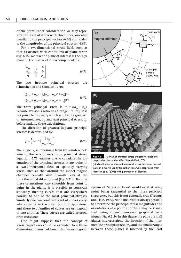
stress, such as that around the model magma
chamber beneath West Spanish Peak at the
time the radial dikes formed (Fig. 6.21a). Because
these orientations vary smoothly from point to
point in the plane, it is possible to construct
smoothly turning curves that are everywhere
parallel to one of the local principal stresses.
Similarly one can construct a set of curves everywhere parallel to the other local principal stress,
and these two families of curves are orthogonal
to one another. These curves are called principal
stress trajectories.
One might suppose that the concept of
stress trajectories could be extended to a threedimensional stress field such that an orthogonal
␥ 1 ϭ
1
2
tan Ϫ1
2 xy
xx Ϫ yy
1
2
1
2 ( xx ϩ yy ) Ϫ [
1
4 ( xx Ϫ yy ) 2 ϩ 2
xy ] 1ր2
1
2 ( xx ϩ yy ) ϩ [
1
4 ( xx Ϫ yy ) 2 ϩ 2
xy ] 1ր2
΄
xx xy 0
yx yy 0
0
0
zz
΅
system of “stress surfaces” would exist at every
point being tangential to the three principal
stress axes, but this is not generally true (Treagus
and Lisle, 1997). None-the-less it is always possible
to determine the principal stress magnitudes and
orientations at a point and these may be visualized using three-dimensional graphical techniques (Fig. 6.21b). In this figure the pairs of small
planes intersect along the direction of the intermediate principal stress, 2 , and the smaller angle
between these planes is bisected by the least
220
FORCE, TRACTION, AND STRESS
Fig 6.21 (a) Map of principal stress trajectories near the
magma chamber under West Spanish Peak, CO.
(b) Visualization of three-dimensional stress field near normal
faults in a North Sea hydrocarbon reservoir. Reprinted from
Maerten et al. (2002) with permission of Elsevier.
(b)
x
magma chamber
principal
stress
trajectory
host rock
⌼ 1
x
ϩ
x
⌼ 1
⌼ 1
1
1
(a)
parallel to the principal vectors (6.70) and scaled
to the magnitudes of the principal stresses (6.69).
For a two-dimensional stress field, such as
that associated with conditions of plane strain
(Fig. 6.16), we take the plane of interest as the (x, y)plane so the matrix of stress components is:
(6.71)
The two in-plane principal stresses are
(Timoshenko and Goodier, 1970):
(6.72)
The third principal stress is zz ϭ( xx ϩ yy ).
Because Poisson’s ratio has a range 0 ՅՅ , it is
not possible to specify which will be the greatest,
1 , intermediate, 2 , and least principal stress, 3 ,
before making these calculations.
The direction of greatest in-plane principal
stresses is determined by:
(6.73)
The angle ␥ 1 is measured from Ox counterclockwise to the axis of maximum principal stress.
Equation (6.73) enables one to calculate the orientation of the principal stresses at any point in
a two-dimensional field of spatially varying
stress, such as that around the model magma
chamber beneath West Spanish Peak at the
time the radial dikes formed (Fig. 6.21a). Because
these orientations vary smoothly from point to
point in the plane, it is possible to construct
smoothly turning curves that are everywhere
parallel to one of the local principal stresses.
Similarly one can construct a set of curves everywhere parallel to the other local principal stress,
and these two families of curves are orthogonal
to one another. These curves are called principal
stress trajectories.
One might suppose that the concept of
stress trajectories could be extended to a threedimensional stress field such that an orthogonal
␥ 1 ϭ
1
2
tan Ϫ1
2 xy
xx Ϫ yy
1
2
1
2 ( xx ϩ yy ) Ϫ [
1
4 ( xx Ϫ yy ) 2 ϩ 2
xy ] 1ր2
1
2 ( xx ϩ yy ) ϩ [
1
4 ( xx Ϫ yy ) 2 ϩ 2
xy ] 1ր2
΄
xx xy 0
yx yy 0
0
0
zz
΅
system of “stress surfaces” would exist at every
point being tangential to the three principal
stress axes, but this is not generally true (Treagus
and Lisle, 1997). None-the-less it is always possible
to determine the principal stress magnitudes and
orientations at a point and these may be visualized using three-dimensional graphical techniques (Fig. 6.21b). In this figure the pairs of small
planes intersect along the direction of the intermediate principal stress, 2 , and the smaller angle
between these planes is bisected by the least
220
FORCE, TRACTION, AND STRESS
Fig 6.21 (a) Map of principal stress trajectories near the
magma chamber under West Spanish Peak, CO.
(b) Visualization of three-dimensional stress field near normal
faults in a North Sea hydrocarbon reservoir. Reprinted from
Maerten et al. (2002) with permission of Elsevier.
(b)
x
magma chamber
principal
stress
trajectory
host rock
⌼ 1
x
ϩ
x
⌼ 1
⌼ 1
1
1
(a)