

6.20a). The complete stress analysis, including
principal stresses, trajectories, and all components, is shown in color on the textbook website.
Equations (6.57) may be solved using matrix
algebra and this is a classic problem called an
eigenvalue problem, which has many applications
in the sciences and engineering (Gere and Weaver,
1965). Here we refer to this as a principal value
problem since we are looking for the principal
values of stress, and (6.57) is written:
(6.65)
A solution to (6.65) is the vector n with components (n x , n y , n z ), which determines the orientation
of a principal plane with respect to the Cartesian
coordinates (x, y, z). The product of the matrix of
stress components and the unit normal components is equal to the product of a scalar, nn , and
the unit normal components, where this scalar is
the unknown principal stress. Rearranging (6.65)
we have the following homogeneous equation:
(6.66)
This equation is called homogeneous because the
right-hand side is the null vector. The second
matrix on the left-hand side is called the identity
matrix because multiplication of a matrix of the
same order by it results in the same matrix.
Carrying out the multiplication and subtraction indicated in (6.66) we have the set of equations (6.57) in matrix form:
(6.67)
One solution to (6.67) is the null vector n, referred
to as a trivial solution, but this is of no interest for
the physical problem we are considering. Nontrivial solutions exist only if the determinant of
the coefficient matrix is zero, as stated in (6.58),
and this leads to the cubic equation (6.59) in the
unknown normal stress, nn . This equation has
΄
xx Ϫ nn
yx
zx
xy
yy Ϫ nn
zy
xz
yz
zz Ϫ nn
΅΄
n x
n y
n z
΅
ϭ
΄
0
0
0 ΅
΄
xx yx zx
xy yy zy
xz yz zz
΅
Ϫ nn
΄
1 0 0
0 1 0
0 0 1 ΅΄
n x
n y
n z
΅
ϭ
΄
0
0
0 ΅
΄
xx yx zx
xy yy zy
xz yz zz
΅΄
n x
n y
n z
΅
ϭ nn ΄
n x
n y
n z
΅
three roots that are the so-called eigenvalues or, as
we refer to them in this context, the principal
values 1 , 2 , 3 . The eigenvalues of an asymmetric matrix can be real or complex, but the special
case of a symmetric matrix always yields real
eigenvalues (Gere and Weaver, 1965), so the symmetric matrix of stress components always yields
real principal stresses. Real eigenvalues may be
positive, negative, or zero and likewise the principal stresses may be positive (tension), negative
(compression), or zero subject only to the constraint that
Each eigenvalue of a matrix is associated with
a vector called the eigenvector. For the matrix of
stress components the eigenvectors are the unit
normal vectors for the planes on which the principal stresses act. Having determined the values of
the three principal stresses from solving (6.59),
these are substituted separately into (6.67) to
obtain three simultaneous equations to be solved
for the components of the normal vector n(1), n(2),
or n(3), associated with each principal stress. In
general, the eigenvectors for a symmetric matrix
are orthogonal to one another (Gere and Weaver,
1965).
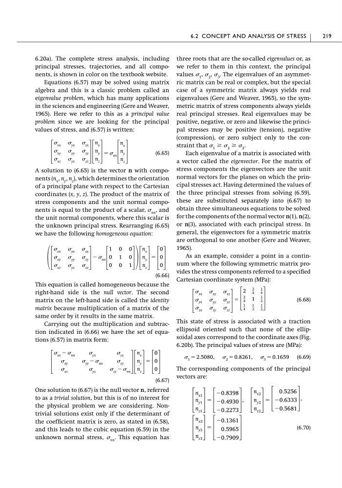
As an example, consider a point in a continuum where the following symmetric matrix provides the stress components referred to a specified
Cartesian coordinate system (MPa):
(6.68)
This state of stress is associated with a traction
ellipsoid oriented such that none of the ellipsoidal axes correspond to the coordinate axes (Fig.
6.20b). The principal values of stress are (MPa):
(6.69)
The corresponding components of the principal
vectors are:
(6.70)
΄
n x3
n y3
n z3
΅
ϭ
΄
Ϫ0.1361
0.5965
Ϫ0.7909
΅
΄
n x1
n y1
n z1
΅
ϭ
΄
Ϫ0.8398
Ϫ0.4930
Ϫ0.2273
΅
,
΄
n x2
n y2
n z2
΅
ϭ
΄
0.5256
Ϫ0.6333
Ϫ0.5681
΅
,
1 ϭ 2.5080, 2 ϭ 0.8261, 3 ϭ 0.1659
΄
xx xy xz
yx yy yz
zx zy zz
΅
ϭ
΄
2
3
4
1
4
3
4
1
1
2
1
4
1
2
1
2
΅
1 Ն 2 Ն 3 .
6.2 CONCEPT AND ANALYSIS OF STRESS
219
principal stresses, trajectories, and all components, is shown in color on the textbook website.
Equations (6.57) may be solved using matrix
algebra and this is a classic problem called an
eigenvalue problem, which has many applications
in the sciences and engineering (Gere and Weaver,
1965). Here we refer to this as a principal value
problem since we are looking for the principal
values of stress, and (6.57) is written:
(6.65)
A solution to (6.65) is the vector n with components (n x , n y , n z ), which determines the orientation
of a principal plane with respect to the Cartesian
coordinates (x, y, z). The product of the matrix of
stress components and the unit normal components is equal to the product of a scalar, nn , and
the unit normal components, where this scalar is
the unknown principal stress. Rearranging (6.65)
we have the following homogeneous equation:
(6.66)
This equation is called homogeneous because the
right-hand side is the null vector. The second
matrix on the left-hand side is called the identity
matrix because multiplication of a matrix of the
same order by it results in the same matrix.
Carrying out the multiplication and subtraction indicated in (6.66) we have the set of equations (6.57) in matrix form:
(6.67)
One solution to (6.67) is the null vector n, referred
to as a trivial solution, but this is of no interest for
the physical problem we are considering. Nontrivial solutions exist only if the determinant of
the coefficient matrix is zero, as stated in (6.58),
and this leads to the cubic equation (6.59) in the
unknown normal stress, nn . This equation has
΄
xx Ϫ nn
yx
zx
xy
yy Ϫ nn
zy
xz
yz
zz Ϫ nn
΅΄
n x
n y
n z
΅
ϭ
΄
0
0
0 ΅
΄
xx yx zx
xy yy zy
xz yz zz
΅
Ϫ nn
΄
1 0 0
0 1 0
0 0 1 ΅΄
n x
n y
n z
΅
ϭ
΄
0
0
0 ΅
΄
xx yx zx
xy yy zy
xz yz zz
΅΄
n x
n y
n z
΅
ϭ nn ΄
n x
n y
n z
΅
three roots that are the so-called eigenvalues or, as
we refer to them in this context, the principal
values 1 , 2 , 3 . The eigenvalues of an asymmetric matrix can be real or complex, but the special
case of a symmetric matrix always yields real
eigenvalues (Gere and Weaver, 1965), so the symmetric matrix of stress components always yields
real principal stresses. Real eigenvalues may be
positive, negative, or zero and likewise the principal stresses may be positive (tension), negative
(compression), or zero subject only to the constraint that
Each eigenvalue of a matrix is associated with
a vector called the eigenvector. For the matrix of
stress components the eigenvectors are the unit
normal vectors for the planes on which the principal stresses act. Having determined the values of
the three principal stresses from solving (6.59),
these are substituted separately into (6.67) to
obtain three simultaneous equations to be solved
for the components of the normal vector n(1), n(2),
or n(3), associated with each principal stress. In
general, the eigenvectors for a symmetric matrix
are orthogonal to one another (Gere and Weaver,
1965).
As an example, consider a point in a continuum where the following symmetric matrix provides the stress components referred to a specified
Cartesian coordinate system (MPa):
(6.68)
This state of stress is associated with a traction
ellipsoid oriented such that none of the ellipsoidal axes correspond to the coordinate axes (Fig.
6.20b). The principal values of stress are (MPa):
(6.69)
The corresponding components of the principal
vectors are:
(6.70)
΄
n x3
n y3
n z3
΅
ϭ
΄
Ϫ0.1361
0.5965
Ϫ0.7909
΅
΄
n x1
n y1
n z1
΅
ϭ
΄
Ϫ0.8398
Ϫ0.4930
Ϫ0.2273
΅
,
΄
n x2
n y2
n z2
΅
ϭ
΄
0.5256
Ϫ0.6333
Ϫ0.5681
΅
,
1 ϭ 2.5080, 2 ϭ 0.8261, 3 ϭ 0.1659
΄
xx xy xz
yx yy yz
zx zy zz
΅
ϭ
΄
2
3
4
1
4
3
4
1
1
2
1
4
1
2
1
2
΅
1 Ն 2 Ն 3 .
6.2 CONCEPT AND ANALYSIS OF STRESS
219