

related to one another such that n x ϭ cos ␣ x and
n y ϭ cos[(/2)Ϫ␣ x ] ϭ sin ␣ x , so the two-dimensional
form of Cauchy’s Formula is:
(6.45)
Here ␣ x is the counterclockwise angle measured
from the Ox-axis to the outward unit normal n for
the plane on which t(n) acts.
6.2.3 Normal and shear tractions on a
surface
For some problems in structural geology it is necessary to calculate the normal and tangential
(shear) traction components acting on an arbitrarily oriented surface within the rock mass as a
function of a homogeneous state of stress. For
example, slip on a fault may be thought of as a
frictional sliding process that is driven by the
shear component of the traction vector acting on
the fault surface (Wallace, 1951; Bott, 1959;
Morris et al., 1996). To the extent that the rock
mass on one side of a fault pushes against the
adjacent fault surface the corresponding (negative) normal component of the traction deters
frictional sliding. Thus, for a set of faults with the
same frictional strength, those carrying the
greatest shear traction and the least (negative)
normal traction would be favored for slip. As a
second example, opening of a joint may be
thought of as driven by the pull of the adjacent
rock mass on the prospective fracture surface
(Pollard and Aydin, 1988). For a rock mass that is
isotropic with respect to tensile strength the
surface with the greatest (positive) normal traction would be favored for jointing.
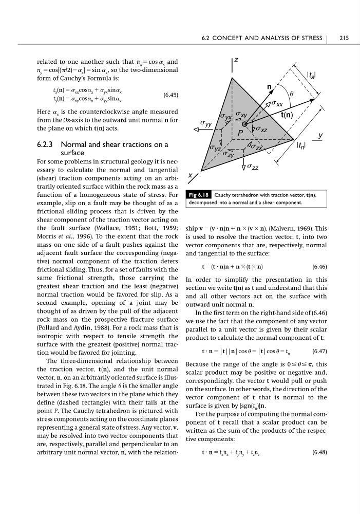
The three-dimensional relationship between
the traction vector, t(n), and the unit normal
vector, n, on an arbitrarily oriented surface is illustrated in Fig. 6.18. The angle is the smaller angle
between these two vectors in the plane which they
define (dashed rectangle) with their tails at the
point P. The Cauchy tetrahedron is pictured with
stress components acting on the coordinate planes
representing a general state of stress. Any vector, v,
may be resolved into two vector components that
are, respectively, parallel and perpendicular to an
arbitrary unit normal vector, n, with the relationt x (n) ϭ xx cos␣ x ϩ yx sin␣ x
t y (n) ϭ xy cos␣ x ϩ yy sin␣ x
ship
(Malvern, 1969). This
is used to resolve the traction vector, t, into two
vector components that are, respectively, normal
and tangential to the surface:
(6.46)
In order to simplify the presentation in this
section we write t(n) as t and understand that this
and all other vectors act on the surface with
outward unit normal n.
In the first term on the right-hand side of (6.46)
we use the fact that the component of any vector
parallel to a unit vector is given by their scalar
product to calculate the normal component of t:
(6.47)
Because the range of the angle is 0 Յ Յ , this
scalar product may be positive or negative and,
correspondingly, the vector t would pull or push
on the surface. In other words, the direction of the
vector component of t that is normal to the
surface is given by [sgn(t n )]n.
For the purpose of computing the normal component of t recall that a scalar product can be
written as the sum of the products of the respective components:
(6.48)
t · n ϭ t x n x ϩ t y n y ϩ t z n z
t · n ϭ |t||n| cos ϭ |t| cos ϭ t n
t ϭ (t · n)n ϩ n ϫ (t ϫ n)
v ϭ (v · n)n ϩ n ϫ (v ϫ n),
6.2 CONCEPT AND ANALYSIS OF STRESS
215
Fig 6.18 Cauchy tetrahedron with traction vector, t(n),
decomposed into a normal and a shear component.
x
y
P
z
n
u
t(n)
|t s |
|t n |
s yx
s yz
s yy
s xx
s xz
s xy
s zx
s zy
s zz
n y ϭ cos[(/2)Ϫ␣ x ] ϭ sin ␣ x , so the two-dimensional
form of Cauchy’s Formula is:
(6.45)
Here ␣ x is the counterclockwise angle measured
from the Ox-axis to the outward unit normal n for
the plane on which t(n) acts.
6.2.3 Normal and shear tractions on a
surface
For some problems in structural geology it is necessary to calculate the normal and tangential
(shear) traction components acting on an arbitrarily oriented surface within the rock mass as a
function of a homogeneous state of stress. For
example, slip on a fault may be thought of as a
frictional sliding process that is driven by the
shear component of the traction vector acting on
the fault surface (Wallace, 1951; Bott, 1959;
Morris et al., 1996). To the extent that the rock
mass on one side of a fault pushes against the
adjacent fault surface the corresponding (negative) normal component of the traction deters
frictional sliding. Thus, for a set of faults with the
same frictional strength, those carrying the
greatest shear traction and the least (negative)
normal traction would be favored for slip. As a
second example, opening of a joint may be
thought of as driven by the pull of the adjacent
rock mass on the prospective fracture surface
(Pollard and Aydin, 1988). For a rock mass that is
isotropic with respect to tensile strength the
surface with the greatest (positive) normal traction would be favored for jointing.
The three-dimensional relationship between
the traction vector, t(n), and the unit normal
vector, n, on an arbitrarily oriented surface is illustrated in Fig. 6.18. The angle is the smaller angle
between these two vectors in the plane which they
define (dashed rectangle) with their tails at the
point P. The Cauchy tetrahedron is pictured with
stress components acting on the coordinate planes
representing a general state of stress. Any vector, v,
may be resolved into two vector components that
are, respectively, parallel and perpendicular to an
arbitrary unit normal vector, n, with the relationt x (n) ϭ xx cos␣ x ϩ yx sin␣ x
t y (n) ϭ xy cos␣ x ϩ yy sin␣ x
ship
(Malvern, 1969). This
is used to resolve the traction vector, t, into two
vector components that are, respectively, normal
and tangential to the surface:
(6.46)
In order to simplify the presentation in this
section we write t(n) as t and understand that this
and all other vectors act on the surface with
outward unit normal n.
In the first term on the right-hand side of (6.46)
we use the fact that the component of any vector
parallel to a unit vector is given by their scalar
product to calculate the normal component of t:
(6.47)
Because the range of the angle is 0 Յ Յ , this
scalar product may be positive or negative and,
correspondingly, the vector t would pull or push
on the surface. In other words, the direction of the
vector component of t that is normal to the
surface is given by [sgn(t n )]n.
For the purpose of computing the normal component of t recall that a scalar product can be
written as the sum of the products of the respective components:
(6.48)
t · n ϭ t x n x ϩ t y n y ϩ t z n z
t · n ϭ |t||n| cos ϭ |t| cos ϭ t n
t ϭ (t · n)n ϩ n ϫ (t ϫ n)
v ϭ (v · n)n ϩ n ϫ (v ϫ n),
6.2 CONCEPT AND ANALYSIS OF STRESS
215
Fig 6.18 Cauchy tetrahedron with traction vector, t(n),
decomposed into a normal and a shear component.
x
y
P
z
n
u
t(n)
|t s |
|t n |
s yx
s yz
s yy
s xx
s xz
s xy
s zx
s zy
s zz