

static equilibrium, but these restrictions can be
relaxed. After introducing the conservation of
linear momentum in Chapter 7 we use this physical law alone to derive Cauchy’s Formula, thereby
showing that it is applicable to problems of solid
deformation and fluid flow including body forces
and accelerations.
Cauchy’s Formula is expressed using indicial
notation for the Cartesian coordinates x i as:
(6.41)
Here it is understood that the repeated index on
the right-hand side implies summation over the
range of j. Given the range of i, (6.41) expands to
three equations, one for each component of the
traction vector. Using a matrix representation for
the components of the traction vector, the stress
tensor, and the unit normal vector, Cauchy’s
Formula may be expressed:
(6.42)
Note that the matrix of stress components is the
transpose of (6.37). The matrix representation
(6.42) emphasizes the fact that the stress tensor
can be thought of as a linear operator that gives
the traction vector as a function of the unit
normal vector. The components of stress are consistent with the definition of a second-order tensor
quantity in that they associate a vector (the traction) with any direction in space as determined by
the respective direction cosines (components of
the unit normal vector).
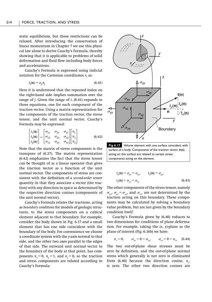
Cauchy’s Formula relates the tractions, acting
as boundary conditions for models of geologic structures, to the stress components on a cubical
element adjacent to that boundary. For example,
consider the body shown in Fig. 6.17 and a small
element that has one side coincident with the
boundary of the body. For convenience we choose
a coordinate system with the y-axis normal to that
side, and the other two axes parallel to the edges
of that side. The outward unit normal vector to
the boundary of the body at that point, has components n x ϭ 0, n y ϭ1, and n z ϭ 0, so the traction
and stress components are related according to
Cauchy’s Formula:
΄
t 1 (n)
t 2 (n)
t 3 (n)
΅
ϭ
΄
11 21 31
12 22 32
13 23 33
΅΄
n 1
n 2
n 3
΅
t i (n) ϭ ji n j
(6.43)
The other components of the stress tensor, namely
xx , xz ϭ zx , and zz , are not determined by the
traction acting on this boundary. These components may be calculated by solving a boundary
value problem, but are not given by the boundary
condition itself.
Cauchy’s Formula given by (6.40) reduces to
two dimensions for conditions of plane deformation. For example, taking the (x, y)-plane as the
plane of interest (Fig. 6.16b) we have:
(6.44)
The two out-of-plane shear stresses must be
zero by definition, and the out-of-plane normal
stress which generally is not zero is eliminated
from (6.40) because the direction cosine, n z ,
is zero. The other two direction cosines are
n z ϭ 0, xz ϭ 0 ϭ zx , yz ϭ 0 ϭ zy
t z (n) ϭ yz ϭ zy
t x (n) ϭ yx ϭ xy , t y (n) ϭ yy ,
214
FORCE, TRACTION, AND STRESS
Fig 6.17 Volume element with one surface coincident with
surface of a body. Components of the traction vector, t(n),
acting on this surface are related to certain stress
components acting on the element.
z
y
x
Boundary
y
z
t(n)
t x (n)
t y (n) t z (n)
n
x
s xx
s zz
s yy
s zx
s zy
s xz
s xy
relaxed. After introducing the conservation of
linear momentum in Chapter 7 we use this physical law alone to derive Cauchy’s Formula, thereby
showing that it is applicable to problems of solid
deformation and fluid flow including body forces
and accelerations.
Cauchy’s Formula is expressed using indicial
notation for the Cartesian coordinates x i as:
(6.41)
Here it is understood that the repeated index on
the right-hand side implies summation over the
range of j. Given the range of i, (6.41) expands to
three equations, one for each component of the
traction vector. Using a matrix representation for
the components of the traction vector, the stress
tensor, and the unit normal vector, Cauchy’s
Formula may be expressed:
(6.42)
Note that the matrix of stress components is the
transpose of (6.37). The matrix representation
(6.42) emphasizes the fact that the stress tensor
can be thought of as a linear operator that gives
the traction vector as a function of the unit
normal vector. The components of stress are consistent with the definition of a second-order tensor
quantity in that they associate a vector (the traction) with any direction in space as determined by
the respective direction cosines (components of
the unit normal vector).
Cauchy’s Formula relates the tractions, acting
as boundary conditions for models of geologic structures, to the stress components on a cubical
element adjacent to that boundary. For example,
consider the body shown in Fig. 6.17 and a small
element that has one side coincident with the
boundary of the body. For convenience we choose
a coordinate system with the y-axis normal to that
side, and the other two axes parallel to the edges
of that side. The outward unit normal vector to
the boundary of the body at that point, has components n x ϭ 0, n y ϭ1, and n z ϭ 0, so the traction
and stress components are related according to
Cauchy’s Formula:
΄
t 1 (n)
t 2 (n)
t 3 (n)
΅
ϭ
΄
11 21 31
12 22 32
13 23 33
΅΄
n 1
n 2
n 3
΅
t i (n) ϭ ji n j
(6.43)
The other components of the stress tensor, namely
xx , xz ϭ zx , and zz , are not determined by the
traction acting on this boundary. These components may be calculated by solving a boundary
value problem, but are not given by the boundary
condition itself.
Cauchy’s Formula given by (6.40) reduces to
two dimensions for conditions of plane deformation. For example, taking the (x, y)-plane as the
plane of interest (Fig. 6.16b) we have:
(6.44)
The two out-of-plane shear stresses must be
zero by definition, and the out-of-plane normal
stress which generally is not zero is eliminated
from (6.40) because the direction cosine, n z ,
is zero. The other two direction cosines are
n z ϭ 0, xz ϭ 0 ϭ zx , yz ϭ 0 ϭ zy
t z (n) ϭ yz ϭ zy
t x (n) ϭ yx ϭ xy , t y (n) ϭ yy ,
214
FORCE, TRACTION, AND STRESS
Fig 6.17 Volume element with one surface coincident with
surface of a body. Components of the traction vector, t(n),
acting on this surface are related to certain stress
components acting on the element.
z
y
x
Boundary
y
z
t(n)
t x (n)
t y (n) t z (n)
n
x
s xx
s zz
s yy
s zx
s zy
s xz
s xy