

ease of representation. One quadrant of the
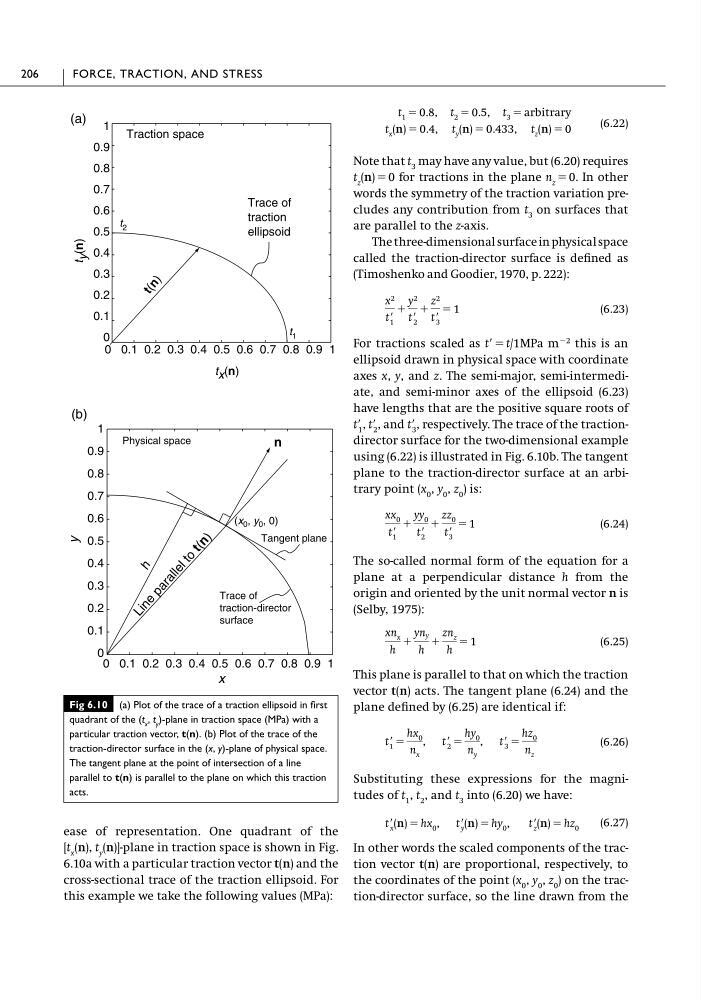
[t x (n), t y (n)]-plane in traction space is shown in Fig.
6.10a with a particular traction vector t(n) and the
cross-sectional trace of the traction ellipsoid. For
this example we take the following values (MPa):
(6.22)
Note that t 3 may have any value, but (6.20) requires
t z (n) ϭ 0 for tractions in the plane n z ϭ 0. In other
words the symmetry of the traction variation precludes any contribution from t 3 on surfaces that
are parallel to the z-axis.
The three-dimensional surface in physical space
called the traction-director surface is defined as
(Timoshenko and Goodier, 1970, p. 222):
(6.23)
For tractions scaled as tЈϭt/1MPa m
Ϫ2 this is an
ellipsoid drawn in physical space with coordinate
axes x, y, and z. The semi-major, semi-intermediate, and semi-minor axes of the ellipsoid (6.23)
have lengths that are the positive square roots of
tЈ 1 , tЈ 2 , and tЈ 3 , respectively. The trace of the tractiondirector surface for the two-dimensional example
using (6.22) is illustrated in Fig. 6.10b. The tangent
plane to the traction-director surface at an arbitrary point (x 0 , y 0 , z 0 ) is:
(6.24)
The so-called normal form of the equation for a
plane at a perpendicular distance h from the
origin and oriented by the unit normal vector n is
(Selby, 1975):
(6.25)
This plane is parallel to that on which the traction
vector t(n) acts. The tangent plane (6.24) and the
plane defined by (6.25) are identical if:
(6.26)
Substituting these expressions for the magnitudes of t 1 , t 2 , and t 3 into (6.20) we have:
(6.27)
In other words the scaled components of the traction vector t(n) are proportional, respectively, to
the coordinates of the point (x 0 , y 0 , z 0 ) on the traction-director surface, so the line drawn from the
tЈ x (n) ϭ hx 0 , tЈ y (n) ϭ hy 0 , tЈ z (n) ϭ hz 0
tЈ 1 ϭ
hx 0
n x
, tЈ 2 ϭ
hy 0
n y
, tЈ 3 ϭ
hz 0
n z
xn x
h
ϩ
yn y
h
ϩ
zn z
h
ϭ 1
xx 0
tЈ 1
ϩ
yy 0
tЈ 2
ϩ
zz 0
tЈ 3
ϭ 1
x 2
tЈ 1
ϩ
y 2
tЈ 2
ϩ
z 2
tЈ 3
ϭ 1
t 1 ϭ 0.8, t 2 ϭ 0.5, t 3 ϭ arbitrary
t x (n) ϭ 0.4,t y (n) ϭ 0.433,t z (n) ϭ 0
206
FORCE, TRACTION, AND STRESS
Fig 6.10 (a) Plot of the trace of a traction ellipsoid in first
quadrant of the (t x , t y )-plane in traction space (MPa) with a
particular traction vector, t(n). (b) Plot of the trace of the
traction-director surface in the (x, y)-plane of physical space.
The tangent plane at the point of intersection of a line
parallel to t(n) is parallel to the plane on which this traction
acts.
Traction space
t 2
Trace of
traction
ellipsoid
t ( n )
t 1
t
y (n)
t x (n)
x
y
Physical space
Tangent plane
Trace of
traction-director
surface
h
L i n e
p a r a l l e l t o
t ( n )
n
(b)
(x 0 , y 0 , 0)
(a) 1
0.9
0.8
0.7
0.6
0.5
0.4
0.3
0.2
0.1
0
0 0.1 0.2 0.3 0.4 0.5 0.6 0.7 0.8 0.9 1
1
0.9
0.8
0.7
0.6
0.5
0.4
0.3
0.2
0.1
0
0 0.1 0.2 0.3 0.4 0.5 0.6 0.7 0.8 0.9 1
[t x (n), t y (n)]-plane in traction space is shown in Fig.
6.10a with a particular traction vector t(n) and the
cross-sectional trace of the traction ellipsoid. For
this example we take the following values (MPa):
(6.22)
Note that t 3 may have any value, but (6.20) requires
t z (n) ϭ 0 for tractions in the plane n z ϭ 0. In other
words the symmetry of the traction variation precludes any contribution from t 3 on surfaces that
are parallel to the z-axis.
The three-dimensional surface in physical space
called the traction-director surface is defined as
(Timoshenko and Goodier, 1970, p. 222):
(6.23)
For tractions scaled as tЈϭt/1MPa m
Ϫ2 this is an
ellipsoid drawn in physical space with coordinate
axes x, y, and z. The semi-major, semi-intermediate, and semi-minor axes of the ellipsoid (6.23)
have lengths that are the positive square roots of
tЈ 1 , tЈ 2 , and tЈ 3 , respectively. The trace of the tractiondirector surface for the two-dimensional example
using (6.22) is illustrated in Fig. 6.10b. The tangent
plane to the traction-director surface at an arbitrary point (x 0 , y 0 , z 0 ) is:
(6.24)
The so-called normal form of the equation for a
plane at a perpendicular distance h from the
origin and oriented by the unit normal vector n is
(Selby, 1975):
(6.25)
This plane is parallel to that on which the traction
vector t(n) acts. The tangent plane (6.24) and the
plane defined by (6.25) are identical if:
(6.26)
Substituting these expressions for the magnitudes of t 1 , t 2 , and t 3 into (6.20) we have:
(6.27)
In other words the scaled components of the traction vector t(n) are proportional, respectively, to
the coordinates of the point (x 0 , y 0 , z 0 ) on the traction-director surface, so the line drawn from the
tЈ x (n) ϭ hx 0 , tЈ y (n) ϭ hy 0 , tЈ z (n) ϭ hz 0
tЈ 1 ϭ
hx 0
n x
, tЈ 2 ϭ
hy 0
n y
, tЈ 3 ϭ
hz 0
n z
xn x
h
ϩ
yn y
h
ϩ
zn z
h
ϭ 1
xx 0
tЈ 1
ϩ
yy 0
tЈ 2
ϩ
zz 0
tЈ 3
ϭ 1
x 2
tЈ 1
ϩ
y 2
tЈ 2
ϩ
z 2
tЈ 3
ϭ 1
t 1 ϭ 0.8, t 2 ϭ 0.5, t 3 ϭ arbitrary
t x (n) ϭ 0.4,t y (n) ϭ 0.433,t z (n) ϭ 0
206
FORCE, TRACTION, AND STRESS
Fig 6.10 (a) Plot of the trace of a traction ellipsoid in first
quadrant of the (t x , t y )-plane in traction space (MPa) with a
particular traction vector, t(n). (b) Plot of the trace of the
traction-director surface in the (x, y)-plane of physical space.
The tangent plane at the point of intersection of a line
parallel to t(n) is parallel to the plane on which this traction
acts.
Traction space
t 2
Trace of
traction
ellipsoid
t ( n )
t 1
t
y (n)
t x (n)
x
y
Physical space
Tangent plane
Trace of
traction-director
surface
h
L i n e
p a r a l l e l t o
t ( n )
n
(b)
(x 0 , y 0 , 0)
(a) 1
0.9
0.8
0.7
0.6
0.5
0.4
0.3
0.2
0.1
0
0 0.1 0.2 0.3 0.4 0.5 0.6 0.7 0.8 0.9 1
1
0.9
0.8
0.7
0.6
0.5
0.4
0.3
0.2
0.1
0
0 0.1 0.2 0.3 0.4 0.5 0.6 0.7 0.8 0.9 1