

Rearranging (6.19), we use (6.18) to eliminate the
areas and write t x (n) ϭ t 1 n x . Here the absolute value
sign in (6.18) has been dropped, so this relationship applies to the full range of orientations of n.
By similar arguments we have:
(6.20)
Note that the components of t(n) have opposite
signs to the respective components of the tractions acting on the orthogonal sides of the
element. Because, for example, the traction Ϫt 1 is
directed in the negative x-direction, the component t x (n) must be positive for a balance of forces.
As the inclined patch rotates toward parallelism
with the (y, z)-plane such that n is directed along
the positive x-axis, we have n x → 1, n y → 0, and
n z → 0 so the y- and z-components of t(n) go to zero
and t x (n) → t 1 , in keeping with (6.9). On the other
hand, as n approaches the negative x-axis, we have
n x → Ϫ1, so t x (n) → Ϫt 1 . Although we derived (6.20)
by ignoring body forces and postulating static
equilibrium, we show in Chapter 7 that this relationship is more generally applicable to problems
of both solid deformation and fluid flow that
include body forces and admit accelerations in
the equations of motion.
The relationships in (6.20) demonstrate that
the traction vector t(n) is equal to the special tractions t 1 , t 2 , and t 3 as n is successively directed in
the positive x-, y-, and z-directions, and it is equal
to Ϫt 1 , Ϫt 2 , and Ϫt 3 as n is successively directed in
the negative x-, y-, and z-directions. But how does
t(n) vary for intermediate orientations? Solving
each of (6.20) for the respective component of the
unit vector and substituting these into (6.17) we
have:
(6.21)
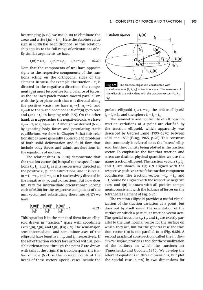
This equation is in the standard form for an ellipsoid drawn in “traction” space with coordinate
axes t x (n), t y (n), and t z (n), (Fig. 6.9). The semi-major,
semi-intermediate, and semi-minor axes of the
ellipsoid have lengths t 1 , t 2 , and t 3 , respectively. If
the set of traction vectors for surfaces with all possible orientations through the point P are drawn
with tails at the origin O in traction space, the traction ellipsoid (6.21) is the locus of points at the
heads of these vectors. Special cases include the
[t x (n)] 2
[t 1 ] 2 ϩ
[t y (n)] 2
[t 2 ] 2 ϩ
[t z (n)] 2
[t 3 ] 2 ϭ 1
t x (n) ϭ t 1 n x ,t y (n) ϭ t 2 n y ,t z (n) ϭ t 3 n z
prolate ellipsoid t 1 Ն t 2 ϭ t 3 , the oblate ellipsoid
t 1 ϭ t 2 Ն t 3 , and the sphere t 1 ϭ t 2 ϭ t 3 .
The symmetry and continuity of all possible
traction variations at a point are clarified by
the traction ellipsoid, which apparently was
described by Gabriel Lamé (1795–1870) between
1820 and 1830 (Fung, 1965, p. 76). This construction commonly is referred to as the “stress” ellipsoid, but the quantity being plotted is the traction
vector. To emphasize the fact that traction and
stress are distinct physical quantities we use the
name traction ellipsoid. The traction vectors t 1 , t 2 ,
and t 3 are shown in Fig. 6.9 aligned with the
respective positive axes of the traction component
coordinates. The traction vectors Ϫt 1 , Ϫt 2 , and
Ϫt 3 would be aligned with the respective negative
axes, and t(n) is drawn with all positive components, consistent with the balance of forces on the
tetrahedral element of Fig. 6.8b.
The traction ellipsoid provides a useful visualization of the traction variation at a point, but
does not by itself reveal the orientation of the
surface on which a particular traction vector acts.
The special tractions t 1 , t 2 , and t 3 are exactly parallel to the unit normal vector for the surface on
which they act, but for the general case the traction vector t(n) is not parallel to n (Fig. 6.8b). A
second graphical construction, called the tractiondirector surface, provides a tool for the visualization
of the surfaces on which the tractions act
(Timoshenko and Goodier, 1970). We develop the
relevant equations in three dimensions, but plot
the special case (n z ϭ 0) in two dimensions for
6.1 CONCEPTS OF FORCE AND TRACTION
205
Fig 6.9 The traction ellipsoid is constructed with
coordinate axes (t x , t y , t z ) in traction space. The semi-axes of
the ellipsoid are coincident with the traction vectors (t 1 , t 2 ,
t 3 ).
Traction space
t y (n)
t x (n)
t z (n)
t 1
t 3
t 2
t(n)
t 1
t 2
t 3
O
areas and write t x (n) ϭ t 1 n x . Here the absolute value
sign in (6.18) has been dropped, so this relationship applies to the full range of orientations of n.
By similar arguments we have:
(6.20)
Note that the components of t(n) have opposite
signs to the respective components of the tractions acting on the orthogonal sides of the
element. Because, for example, the traction Ϫt 1 is
directed in the negative x-direction, the component t x (n) must be positive for a balance of forces.
As the inclined patch rotates toward parallelism
with the (y, z)-plane such that n is directed along
the positive x-axis, we have n x → 1, n y → 0, and
n z → 0 so the y- and z-components of t(n) go to zero
and t x (n) → t 1 , in keeping with (6.9). On the other
hand, as n approaches the negative x-axis, we have
n x → Ϫ1, so t x (n) → Ϫt 1 . Although we derived (6.20)
by ignoring body forces and postulating static
equilibrium, we show in Chapter 7 that this relationship is more generally applicable to problems
of both solid deformation and fluid flow that
include body forces and admit accelerations in
the equations of motion.
The relationships in (6.20) demonstrate that
the traction vector t(n) is equal to the special tractions t 1 , t 2 , and t 3 as n is successively directed in
the positive x-, y-, and z-directions, and it is equal
to Ϫt 1 , Ϫt 2 , and Ϫt 3 as n is successively directed in
the negative x-, y-, and z-directions. But how does
t(n) vary for intermediate orientations? Solving
each of (6.20) for the respective component of the
unit vector and substituting these into (6.17) we
have:
(6.21)
This equation is in the standard form for an ellipsoid drawn in “traction” space with coordinate
axes t x (n), t y (n), and t z (n), (Fig. 6.9). The semi-major,
semi-intermediate, and semi-minor axes of the
ellipsoid have lengths t 1 , t 2 , and t 3 , respectively. If
the set of traction vectors for surfaces with all possible orientations through the point P are drawn
with tails at the origin O in traction space, the traction ellipsoid (6.21) is the locus of points at the
heads of these vectors. Special cases include the
[t x (n)] 2
[t 1 ] 2 ϩ
[t y (n)] 2
[t 2 ] 2 ϩ
[t z (n)] 2
[t 3 ] 2 ϭ 1
t x (n) ϭ t 1 n x ,t y (n) ϭ t 2 n y ,t z (n) ϭ t 3 n z
prolate ellipsoid t 1 Ն t 2 ϭ t 3 , the oblate ellipsoid
t 1 ϭ t 2 Ն t 3 , and the sphere t 1 ϭ t 2 ϭ t 3 .
The symmetry and continuity of all possible
traction variations at a point are clarified by
the traction ellipsoid, which apparently was
described by Gabriel Lamé (1795–1870) between
1820 and 1830 (Fung, 1965, p. 76). This construction commonly is referred to as the “stress” ellipsoid, but the quantity being plotted is the traction
vector. To emphasize the fact that traction and
stress are distinct physical quantities we use the
name traction ellipsoid. The traction vectors t 1 , t 2 ,
and t 3 are shown in Fig. 6.9 aligned with the
respective positive axes of the traction component
coordinates. The traction vectors Ϫt 1 , Ϫt 2 , and
Ϫt 3 would be aligned with the respective negative
axes, and t(n) is drawn with all positive components, consistent with the balance of forces on the
tetrahedral element of Fig. 6.8b.
The traction ellipsoid provides a useful visualization of the traction variation at a point, but
does not by itself reveal the orientation of the
surface on which a particular traction vector acts.
The special tractions t 1 , t 2 , and t 3 are exactly parallel to the unit normal vector for the surface on
which they act, but for the general case the traction vector t(n) is not parallel to n (Fig. 6.8b). A
second graphical construction, called the tractiondirector surface, provides a tool for the visualization
of the surfaces on which the tractions act
(Timoshenko and Goodier, 1970). We develop the
relevant equations in three dimensions, but plot
the special case (n z ϭ 0) in two dimensions for
6.1 CONCEPTS OF FORCE AND TRACTION
205
Fig 6.9 The traction ellipsoid is constructed with
coordinate axes (t x , t y , t z ) in traction space. The semi-axes of
the ellipsoid are coincident with the traction vectors (t 1 , t 2 ,
t 3 ).
Traction space
t y (n)
t x (n)
t z (n)
t 1
t 3
t 2
t(n)
t 1
t 2
t 3
O