

variation of the traction vector with the orientation of n.
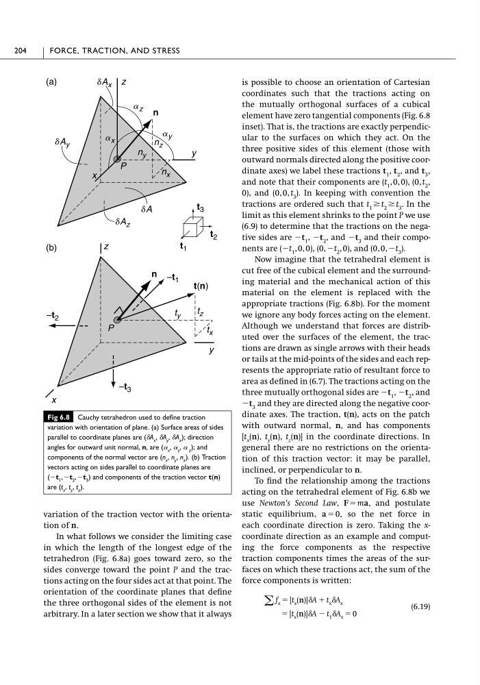
In what follows we consider the limiting case
in which the length of the longest edge of the
tetrahedron (Fig. 6.8a) goes toward zero, so the
sides converge toward the point P and the tractions acting on the four sides act at that point. The
orientation of the coordinate planes that define
the three orthogonal sides of the element is not
arbitrary. In a later section we show that it always
is possible to choose an orientation of Cartesian
coordinates such that the tractions acting on
the mutually orthogonal surfaces of a cubical
element have zero tangential components (Fig. 6.8
inset). That is, the tractions are exactly perpendicular to the surfaces on which they act. On the
three positive sides of this element (those with
outward normals directed along the positive coordinate axes) we label these tractions t 1 , t 2 , and t 3 ,
and note that their components are (t 1 ,0, 0), (0, t 2 ,
0), and (0, 0, t 3 ). In keeping with convention the
tractions are ordered such that t 1 Ն t 2 Ն t 3 . In the
limit as this element shrinks to the point P we use
(6.9) to determine that the tractions on the negative sides are Ϫt 1 , Ϫt 2 , and Ϫt 3 and their components are (Ϫt 1 ,0, 0), (0, Ϫt 2 , 0), and (0, 0, Ϫt 3 ).
Now imagine that the tetrahedral element is
cut free of the cubical element and the surrounding material and the mechanical action of this
material on the element is replaced with the
appropriate tractions (Fig. 6.8b). For the moment
we ignore any body forces acting on the element.
Although we understand that forces are distributed over the surfaces of the element, the tractions are drawn as single arrows with their heads
or tails at the mid-points of the sides and each represents the appropriate ratio of resultant force to
area as defined in (6.7). The tractions acting on the
three mutually orthogonal sides are Ϫt 1 , Ϫt 2 , and
Ϫt 3 and they are directed along the negative coordinate axes. The traction, t(n), acts on the patch
with outward normal, n, and has components
[t x (n), t y (n), t z (n)] in the coordinate directions. In
general there are no restrictions on the orientation of this traction vector: it may be parallel,
inclined, or perpendicular to n.
To find the relationship among the tractions
acting on the tetrahedral element of Fig. 6.8b we
use Newton’s Second Law, F ϭ ma, and postulate
static equilibrium, a ϭ 0, so the net force in
each coordinate direction is zero. Taking the xcoordinate direction as an example and computing the force components as the respective
traction components times the areas of the surfaces on which these tractions act, the sum of the
force components is written:
(6.19)
ϭ [t x (n)]␦A Ϫ t 1 ␦A x ϭ 0
͚ f x ϭ [t x (n)]␦A ϩ t x ␦A x
204
FORCE, TRACTION, AND STRESS
Fig 6.8 Cauchy tetrahedron used to define traction
variation with orientation of plane. (a) Surface areas of sides
parallel to coordinate planes are (␦A x , ␦A y , ␦A z ); direction
angles for outward unit normal, n, are (␣ x , ␣ y , ␣ z ); and
components of the normal vector are (n x , n y , n z ). (b) Traction
vectors acting on sides parallel to coordinate planes are
(Ϫt 1 , Ϫt 2 , Ϫt 3 ) and components of the traction vector t(n)
are (t x , t y , t z ).
–t 1
(a)
x
y
z
n
(b)
–t 3
–t 2
t(n)
t x
t z
t y
dA
n z
n x
n y
x
y
z
n
a x
a z
a y
dA y
P
dA z
dA x
P
t 1
t 2
t 3
In what follows we consider the limiting case
in which the length of the longest edge of the
tetrahedron (Fig. 6.8a) goes toward zero, so the
sides converge toward the point P and the tractions acting on the four sides act at that point. The
orientation of the coordinate planes that define
the three orthogonal sides of the element is not
arbitrary. In a later section we show that it always
is possible to choose an orientation of Cartesian
coordinates such that the tractions acting on
the mutually orthogonal surfaces of a cubical
element have zero tangential components (Fig. 6.8
inset). That is, the tractions are exactly perpendicular to the surfaces on which they act. On the
three positive sides of this element (those with
outward normals directed along the positive coordinate axes) we label these tractions t 1 , t 2 , and t 3 ,
and note that their components are (t 1 ,0, 0), (0, t 2 ,
0), and (0, 0, t 3 ). In keeping with convention the
tractions are ordered such that t 1 Ն t 2 Ն t 3 . In the
limit as this element shrinks to the point P we use
(6.9) to determine that the tractions on the negative sides are Ϫt 1 , Ϫt 2 , and Ϫt 3 and their components are (Ϫt 1 ,0, 0), (0, Ϫt 2 , 0), and (0, 0, Ϫt 3 ).
Now imagine that the tetrahedral element is
cut free of the cubical element and the surrounding material and the mechanical action of this
material on the element is replaced with the
appropriate tractions (Fig. 6.8b). For the moment
we ignore any body forces acting on the element.
Although we understand that forces are distributed over the surfaces of the element, the tractions are drawn as single arrows with their heads
or tails at the mid-points of the sides and each represents the appropriate ratio of resultant force to
area as defined in (6.7). The tractions acting on the
three mutually orthogonal sides are Ϫt 1 , Ϫt 2 , and
Ϫt 3 and they are directed along the negative coordinate axes. The traction, t(n), acts on the patch
with outward normal, n, and has components
[t x (n), t y (n), t z (n)] in the coordinate directions. In
general there are no restrictions on the orientation of this traction vector: it may be parallel,
inclined, or perpendicular to n.
To find the relationship among the tractions
acting on the tetrahedral element of Fig. 6.8b we
use Newton’s Second Law, F ϭ ma, and postulate
static equilibrium, a ϭ 0, so the net force in
each coordinate direction is zero. Taking the xcoordinate direction as an example and computing the force components as the respective
traction components times the areas of the surfaces on which these tractions act, the sum of the
force components is written:
(6.19)
ϭ [t x (n)]␦A Ϫ t 1 ␦A x ϭ 0
͚ f x ϭ [t x (n)]␦A ϩ t x ␦A x
204
FORCE, TRACTION, AND STRESS
Fig 6.8 Cauchy tetrahedron used to define traction
variation with orientation of plane. (a) Surface areas of sides
parallel to coordinate planes are (␦A x , ␦A y , ␦A z ); direction
angles for outward unit normal, n, are (␣ x , ␣ y , ␣ z ); and
components of the normal vector are (n x , n y , n z ). (b) Traction
vectors acting on sides parallel to coordinate planes are
(Ϫt 1 , Ϫt 2 , Ϫt 3 ) and components of the traction vector t(n)
are (t x , t y , t z ).
–t 1
(a)
x
y
z
n
(b)
–t 3
–t 2
t(n)
t x
t z
t y
dA
n z
n x
n y
x
y
z
n
a x
a z
a y
dA y
P
dA z
dA x
P
t 1
t 2
t 3