

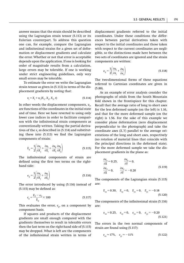
answer means that the strain should be described
using the Lagrangian strain tensor (5.113) or its
Eulerian counterpart. To address this question
one can, for example, compare the Lagrangian
and infinitesimal strains for a given set of deformation or displacement gradients and calculate
the error. Whether or not that error is acceptable
depends upon the application. If one is looking for
order of magnitude results from a calculation,
large errors may be tolerable. If one is working
under strict engineering guidelines, only very
small errors may be tolerable.
To estimate the error we write the Lagrangian
strain tensor as given in (5.113) in terms of the displacement gradients by noting that:
x i ϭ X i ϩ u i (X 1 , X 2 , X 3 , t)
(5.114)
In other words the displacement components, u i ,
are functions of the coordinates in the initial state
and of time. Here we have reverted to using only
lower case indices in order to facilitate comparison with the infinitesimal strain components as
conventionally written. Taking the partial derivatives of the x i as described in (5.114) and substituting these into (5.113) we find the Lagrangian
components of strain:
(5.115)
The infinitesimal components of strain are
defined using the first two terms on the righthand side:
(5.116)
The error introduced by using (5.116) instead of
(5.115) may be defined as:
(5.117)
This evaluates the error, e ij , on a component by
component basis.
If squares and products of the displacement
gradients are small enough compared with the
gradients themselves to result in tolerable errors
then the last term on the right-hand side of (5.115)
may be dropped. What is left are the components
of the infinitesimal strain written in terms of
e ij ϭ
E ij Ϫ ij
E ij
ϫ 100
ij ϭ
1
2
Ѩu i
ѨX j
ϩ
Ѩu j
ѨX i
E ij ϭ
1
2
Ѩu i
ѨX j
ϩ
Ѩu j
ѨX i
ϩ
Ѩu k
ѨX i
Ѩu k
ѨX j
displacement gradients referred to the initial
coordinates. Under these conditions the differences between partial derivatives taken with
respect to the initial coordinates and those taken
with respect to the current coordinates are negligible, so the distinctions made here between the
two sets of coordinates are ignored and the strain
components are written:
(5.118)
The two-dimensional forms of these equations
referred to Cartesian coordinates are given in
(5.88).
As an example of error analysis consider the
photographs of oöids from the South Mountain
fold shown in the frontispiece for this chapter.
Recall that the average ratio of long to short axes
for the less deformed sample (on the left) is 1.16,
and that for the more deformed sample (on the
right) is 1.56. For the sake of this example we
consider plane deformation (zero displacement
perpendicular to the photograph) and take the
coordinate axes (X, Y) parallel to the average orientations of the long and short axes, respectively
(no rotation of material lines that coincide with
the principal directions in the deformed state).
For the more deformed sample we take the displacement gradients in the plane as:
(5.119)
The components of the Lagrangian strain (5.115)
are:
E xx ϭ 0.30, E xy ϭ 0, E yx ϭ 0, E yy ϭϪ0.18
(5.120)
The components of the infinitesimal strain (5.116)
are:
xx ϭ 0.25, xy ϭ 0, yx ϭ 0, yy ϭϪ0.20
(5.121)
The errors in the two normal components of
strain are found using (5.117):
e xx Ϸ 17%, e yy Ϸ Ϫ11%
(5.122)
Ѩu y
ѨX
ϭ 0,
Ѩu y
ѨY
ϭ Ϫ0.20
Ѩu x
ѨX
ϭ 0.25,
Ѩu x
ѨY
ϭ 0,
ij ϭ
1
2
Ѩu i
Ѩx j
ϩ
Ѩu j
Ѩx i
5.5 GENERAL RESULTS
191
using the Lagrangian strain tensor (5.113) or its
Eulerian counterpart. To address this question
one can, for example, compare the Lagrangian
and infinitesimal strains for a given set of deformation or displacement gradients and calculate
the error. Whether or not that error is acceptable
depends upon the application. If one is looking for
order of magnitude results from a calculation,
large errors may be tolerable. If one is working
under strict engineering guidelines, only very
small errors may be tolerable.
To estimate the error we write the Lagrangian
strain tensor as given in (5.113) in terms of the displacement gradients by noting that:
x i ϭ X i ϩ u i (X 1 , X 2 , X 3 , t)
(5.114)
In other words the displacement components, u i ,
are functions of the coordinates in the initial state
and of time. Here we have reverted to using only
lower case indices in order to facilitate comparison with the infinitesimal strain components as
conventionally written. Taking the partial derivatives of the x i as described in (5.114) and substituting these into (5.113) we find the Lagrangian
components of strain:
(5.115)
The infinitesimal components of strain are
defined using the first two terms on the righthand side:
(5.116)
The error introduced by using (5.116) instead of
(5.115) may be defined as:
(5.117)
This evaluates the error, e ij , on a component by
component basis.
If squares and products of the displacement
gradients are small enough compared with the
gradients themselves to result in tolerable errors
then the last term on the right-hand side of (5.115)
may be dropped. What is left are the components
of the infinitesimal strain written in terms of
e ij ϭ
E ij Ϫ ij
E ij
ϫ 100
ij ϭ
1
2
Ѩu i
ѨX j
ϩ
Ѩu j
ѨX i
E ij ϭ
1
2
Ѩu i
ѨX j
ϩ
Ѩu j
ѨX i
ϩ
Ѩu k
ѨX i
Ѩu k
ѨX j
displacement gradients referred to the initial
coordinates. Under these conditions the differences between partial derivatives taken with
respect to the initial coordinates and those taken
with respect to the current coordinates are negligible, so the distinctions made here between the
two sets of coordinates are ignored and the strain
components are written:
(5.118)
The two-dimensional forms of these equations
referred to Cartesian coordinates are given in
(5.88).
As an example of error analysis consider the
photographs of oöids from the South Mountain
fold shown in the frontispiece for this chapter.
Recall that the average ratio of long to short axes
for the less deformed sample (on the left) is 1.16,
and that for the more deformed sample (on the
right) is 1.56. For the sake of this example we
consider plane deformation (zero displacement
perpendicular to the photograph) and take the
coordinate axes (X, Y) parallel to the average orientations of the long and short axes, respectively
(no rotation of material lines that coincide with
the principal directions in the deformed state).
For the more deformed sample we take the displacement gradients in the plane as:
(5.119)
The components of the Lagrangian strain (5.115)
are:
E xx ϭ 0.30, E xy ϭ 0, E yx ϭ 0, E yy ϭϪ0.18
(5.120)
The components of the infinitesimal strain (5.116)
are:
xx ϭ 0.25, xy ϭ 0, yx ϭ 0, yy ϭϪ0.20
(5.121)
The errors in the two normal components of
strain are found using (5.117):
e xx Ϸ 17%, e yy Ϸ Ϫ11%
(5.122)
Ѩu y
ѨX
ϭ 0,
Ѩu y
ѨY
ϭ Ϫ0.20
Ѩu x
ѨX
ϭ 0.25,
Ѩu x
ѨY
ϭ 0,
ij ϭ
1
2
Ѩu i
Ѩx j
ϩ
Ѩu j
Ѩx i
5.5 GENERAL RESULTS
191