

application in models for the formation of joints,
dikes, faults, or other structures.
Notice that there are two applications of the
“infinitesimal concept” in the preceding discussion. The first is introduced in calculus and concerns the treatment of a material line element
of arbitrary orientation that is represented by
the infinitesimal vector dX with components
(dX, dY) in the initial state and dx with components (dx, dy) in the deformed state. These
vectors are contained within a neighborhood of
the particle or spatial point from which they
emanate that is sufficiently small so one may
ignore the non-linear terms in the Taylor series
expansion about that particle or point. For
example we have:
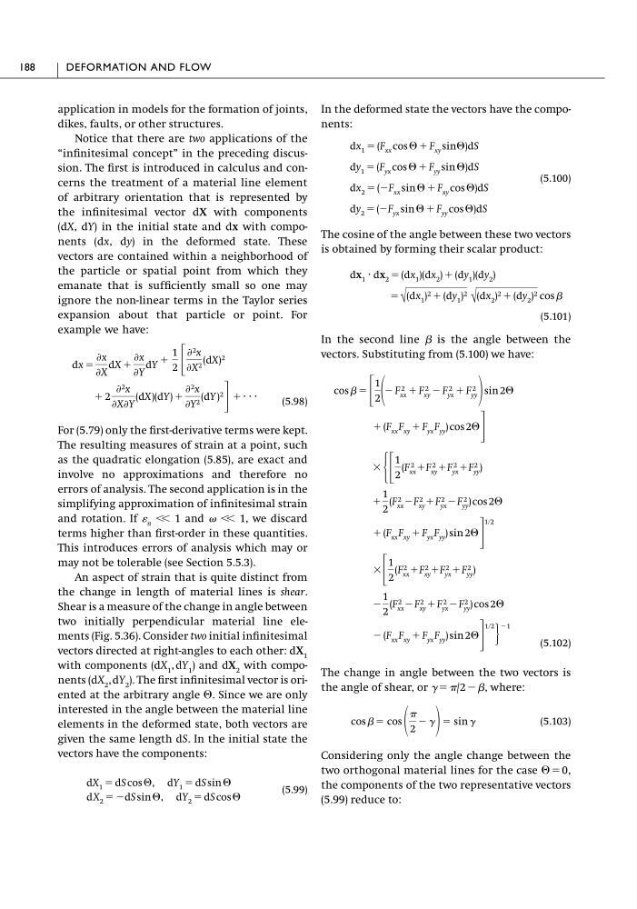
(5.98)
For (5.79) only the first-derivative terms were kept.
The resulting measures of strain at a point, such
as the quadratic elongation (5.85), are exact and
involve no approximations and therefore no
errors of analysis. The second application is in the
simplifying approximation of infinitesimal strain
and rotation. If n Ͻ Ͻ 1 and Ͻ Ͻ 1, we discard
terms higher than first-order in these quantities.
This introduces errors of analysis which may or
may not be tolerable (see Section 5.5.3).
An aspect of strain that is quite distinct from
the change in length of material lines is shear.
Shear is a measure of the change in angle between
two initially perpendicular material line elements (Fig. 5.36). Consider two initial infinitesimal
vectors directed at right-angles to each other: dX 1
with components (dX 1 ,dY 1 ) and dX 2 with components (dX 2 ,dY 2 ). The first infinitesimal vector is oriented at the arbitrary angle ⌰. Since we are only
interested in the angle between the material line
elements in the deformed state, both vectors are
given the same length dS. In the initial state the
vectors have the components:
(5.99)
dX 2 ϭ ϪdS sin ⌰, dY 2 ϭ dS cos ⌰
dX 1 ϭ dS cos ⌰, dY 1 ϭ dS sin ⌰
ϩ 2
Ѩ 2 x
ѨXѨY
(dX)(dY) ϩ
Ѩ 2 x
ѨY 2 (dY ) 2
΅
ϩ · · ·
ϩ
1
2 ΄
Ѩ 2 x
ѨX 2 (dX) 2
dx ϭ
Ѩx
ѨX
dX ϩ
Ѩx
ѨY
dY
In the deformed state the vectors have the components:
(5.100)
The cosine of the angle between these two vectors
is obtained by forming their scalar product:
(5.101)
In the second line  is the angle between the
vectors. Substituting from (5.100) we have:
(5.102)
The change in angle between the two vectors is
the angle of shear, or ␥ ϭ /2 Ϫ , where:
(5.103)
Considering only the angle change between the
two orthogonal material lines for the case ⌰ϭ0,
the components of the two representative vectors
(5.99) reduce to:
cos  ϭ cos
2
Ϫ ␥ ϭ sin ␥
Ϫ (F xx F xy ϩ F yx F yy ) sin 2⌰
΅
1ր2
·
Ϫ1
Ϫ
1
2
(F 2
xx ϪF 2
xy ϩF 2
yx ϪF 2
yy ) cos 2⌰
ϫ
΄
1
2
(F 2
xx ϩF 2
xy ϩF 2
yx ϩF 2
yy )
ϩ (F xx F xy ϩ F yx F yy ) sin 2⌰
΅
1ր2
ϩ
1
2
(F 2
xx ϪF 2
xy ϩF 2
yx ϪF 2
yy ) cos 2⌰
ϫ
Ά΄
1
2
(F 2
xx ϩF 2
xy ϩF 2
yx ϩF 2
yy )
ϩ (F xx F xy ϩ F yx F yy ) cos 2⌰ ΅
cos  ϭ ΄
1
2 Ϫ F 2
xx ϩ F 2
xy Ϫ F 2
yx ϩ F 2
yy sin 2⌰
ϭ √ (dx 1 ) 2 ϩ (dy 1 ) 2 √ (dx 2 ) 2 ϩ (dy 2 ) 2 cos 
dx 1 · dx 2 ϭ (dx 1 )(dx 2 ) ϩ (dy 1 )(dy 2 )
dy 2 ϭ (ϪF yx sin ⌰ ϩ F yy cos ⌰)dS
dx 2 ϭ ( ϪF xx sin ⌰ ϩ F xy cos ⌰)dS
dy 1 ϭ (F yx cos ⌰ ϩ F yy sin ⌰)dS
dx 1 ϭ (F xx cos ⌰ ϩ F xy sin⌰)dS
188
DEFORMATION AND FLOW
dikes, faults, or other structures.
Notice that there are two applications of the
“infinitesimal concept” in the preceding discussion. The first is introduced in calculus and concerns the treatment of a material line element
of arbitrary orientation that is represented by
the infinitesimal vector dX with components
(dX, dY) in the initial state and dx with components (dx, dy) in the deformed state. These
vectors are contained within a neighborhood of
the particle or spatial point from which they
emanate that is sufficiently small so one may
ignore the non-linear terms in the Taylor series
expansion about that particle or point. For
example we have:
(5.98)
For (5.79) only the first-derivative terms were kept.
The resulting measures of strain at a point, such
as the quadratic elongation (5.85), are exact and
involve no approximations and therefore no
errors of analysis. The second application is in the
simplifying approximation of infinitesimal strain
and rotation. If n Ͻ Ͻ 1 and Ͻ Ͻ 1, we discard
terms higher than first-order in these quantities.
This introduces errors of analysis which may or
may not be tolerable (see Section 5.5.3).
An aspect of strain that is quite distinct from
the change in length of material lines is shear.
Shear is a measure of the change in angle between
two initially perpendicular material line elements (Fig. 5.36). Consider two initial infinitesimal
vectors directed at right-angles to each other: dX 1
with components (dX 1 ,dY 1 ) and dX 2 with components (dX 2 ,dY 2 ). The first infinitesimal vector is oriented at the arbitrary angle ⌰. Since we are only
interested in the angle between the material line
elements in the deformed state, both vectors are
given the same length dS. In the initial state the
vectors have the components:
(5.99)
dX 2 ϭ ϪdS sin ⌰, dY 2 ϭ dS cos ⌰
dX 1 ϭ dS cos ⌰, dY 1 ϭ dS sin ⌰
ϩ 2
Ѩ 2 x
ѨXѨY
(dX)(dY) ϩ
Ѩ 2 x
ѨY 2 (dY ) 2
΅
ϩ · · ·
ϩ
1
2 ΄
Ѩ 2 x
ѨX 2 (dX) 2
dx ϭ
Ѩx
ѨX
dX ϩ
Ѩx
ѨY
dY
In the deformed state the vectors have the components:
(5.100)
The cosine of the angle between these two vectors
is obtained by forming their scalar product:
(5.101)
In the second line  is the angle between the
vectors. Substituting from (5.100) we have:
(5.102)
The change in angle between the two vectors is
the angle of shear, or ␥ ϭ /2 Ϫ , where:
(5.103)
Considering only the angle change between the
two orthogonal material lines for the case ⌰ϭ0,
the components of the two representative vectors
(5.99) reduce to:
cos  ϭ cos
2
Ϫ ␥ ϭ sin ␥
Ϫ (F xx F xy ϩ F yx F yy ) sin 2⌰
΅
1ր2
·
Ϫ1
Ϫ
1
2
(F 2
xx ϪF 2
xy ϩF 2
yx ϪF 2
yy ) cos 2⌰
ϫ
΄
1
2
(F 2
xx ϩF 2
xy ϩF 2
yx ϩF 2
yy )
ϩ (F xx F xy ϩ F yx F yy ) sin 2⌰
΅
1ր2
ϩ
1
2
(F 2
xx ϪF 2
xy ϩF 2
yx ϪF 2
yy ) cos 2⌰
ϫ
Ά΄
1
2
(F 2
xx ϩF 2
xy ϩF 2
yx ϩF 2
yy )
ϩ (F xx F xy ϩ F yx F yy ) cos 2⌰ ΅
cos  ϭ ΄
1
2 Ϫ F 2
xx ϩ F 2
xy Ϫ F 2
yx ϩ F 2
yy sin 2⌰
ϭ √ (dx 1 ) 2 ϩ (dy 1 ) 2 √ (dx 2 ) 2 ϩ (dy 2 ) 2 cos 
dx 1 · dx 2 ϭ (dx 1 )(dx 2 ) ϩ (dy 1 )(dy 2 )
dy 2 ϭ (ϪF yx sin ⌰ ϩ F yy cos ⌰)dS
dx 2 ϭ ( ϪF xx sin ⌰ ϩ F xy cos ⌰)dS
dy 1 ϭ (F yx cos ⌰ ϩ F yy sin ⌰)dS
dx 1 ϭ (F xx cos ⌰ ϩ F xy sin⌰)dS
188
DEFORMATION AND FLOW