

Here ␦(t) is required to define the velocity field for
the general model. This method uses quantities
evaluated at the initial position of the particle.
Since the velocity will generally change continuously between the initial and final positions, a
gradual divergence between the computed trajectory of the particle and the true trajectory may
develop. To minimize this, we use small time
increments. Alternatively, the velocity may be
computed at the new position, and the average
velocity for the two positions used to re-compute
the new position. This method involves a slightly
lengthier computer program, but it provides
more stable results. In the present examples this
refined method is not used.
Following individual particles may be informative, such as convective motion in a magma
chamber. We will often follow particle loci that
allow us to visualize the velocity field or the
current state of deformation. Such initial loci for
two-dimensional motions might be circles or
lines; for three-dimensional motions, they might
be spherical surfaces, planes, or lines. These are
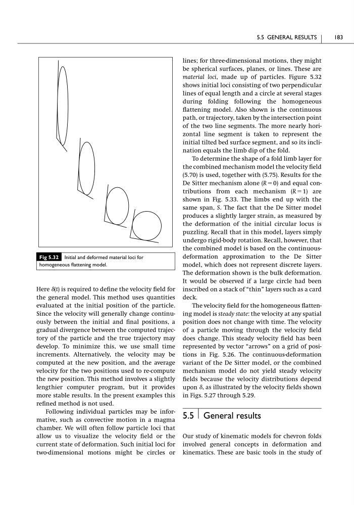
material loci, made up of particles. Figure 5.32
shows initial loci consisting of two perpendicular
lines of equal length and a circle at several stages
during folding following the homogeneous
flattening model. Also shown is the continuous
path, or trajectory, taken by the intersection point
of the two line segments. The more nearly horizontal line segment is taken to represent the
initial tilted bed surface segment, and so its inclination equals the limb dip of the fold.
To determine the shape of a fold limb layer for
the combined mechanism model the velocity field
(5.70) is used, together with (5.75). Results for the
De Sitter mechanism alone (R ϭ 0) and equal contributions from each mechanism (R ϭ 1) are
shown in Fig. 5.33. The limbs end up with the
same span, S. The fact that the De Sitter model
produces a slightly larger strain, as measured by
the deformation of the initial circular locus is
puzzling. Recall that in this model, layers simply
undergo rigid-body rotation. Recall, however, that
the combined model is based on the continuousdeformation approximation to the De Sitter
model, which does not represent discrete layers.
The deformation shown is the bulk deformation.
It would be observed if a large circle had been
inscribed on a stack of “thin” layers such as a card
deck.
The velocity field for the homogeneous flattening model is steady state: the velocity at any spatial
position does not change with time. The velocity
of a particle moving through the velocity field
does change. This steady velocity field has been
represented by vector “arrows” on a grid of positions in Fig. 5.26. The continuous-deformation
variant of the De Sitter model, or the combined
mechanism model do not yield steady velocity
fields because the velocity distributions depend
upon ␦, as illustrated by the velocity fields shown
in Figs. 5.27 through 5.29.
5.5 General results
Our study of kinematic models for chevron folds
involved general concepts in deformation and
kinematics. These are basic tools in the study of
5.5 GENERAL RESULTS
183
Fig 5.32 Initial and deformed material loci for
homogeneous flattening model.
the general model. This method uses quantities
evaluated at the initial position of the particle.
Since the velocity will generally change continuously between the initial and final positions, a
gradual divergence between the computed trajectory of the particle and the true trajectory may
develop. To minimize this, we use small time
increments. Alternatively, the velocity may be
computed at the new position, and the average
velocity for the two positions used to re-compute
the new position. This method involves a slightly
lengthier computer program, but it provides
more stable results. In the present examples this
refined method is not used.
Following individual particles may be informative, such as convective motion in a magma
chamber. We will often follow particle loci that
allow us to visualize the velocity field or the
current state of deformation. Such initial loci for
two-dimensional motions might be circles or
lines; for three-dimensional motions, they might
be spherical surfaces, planes, or lines. These are
material loci, made up of particles. Figure 5.32
shows initial loci consisting of two perpendicular
lines of equal length and a circle at several stages
during folding following the homogeneous
flattening model. Also shown is the continuous
path, or trajectory, taken by the intersection point
of the two line segments. The more nearly horizontal line segment is taken to represent the
initial tilted bed surface segment, and so its inclination equals the limb dip of the fold.
To determine the shape of a fold limb layer for
the combined mechanism model the velocity field
(5.70) is used, together with (5.75). Results for the
De Sitter mechanism alone (R ϭ 0) and equal contributions from each mechanism (R ϭ 1) are
shown in Fig. 5.33. The limbs end up with the
same span, S. The fact that the De Sitter model
produces a slightly larger strain, as measured by
the deformation of the initial circular locus is
puzzling. Recall that in this model, layers simply
undergo rigid-body rotation. Recall, however, that
the combined model is based on the continuousdeformation approximation to the De Sitter
model, which does not represent discrete layers.
The deformation shown is the bulk deformation.
It would be observed if a large circle had been
inscribed on a stack of “thin” layers such as a card
deck.
The velocity field for the homogeneous flattening model is steady state: the velocity at any spatial
position does not change with time. The velocity
of a particle moving through the velocity field
does change. This steady velocity field has been
represented by vector “arrows” on a grid of positions in Fig. 5.26. The continuous-deformation
variant of the De Sitter model, or the combined
mechanism model do not yield steady velocity
fields because the velocity distributions depend
upon ␦, as illustrated by the velocity fields shown
in Figs. 5.27 through 5.29.
5.5 General results
Our study of kinematic models for chevron folds
involved general concepts in deformation and
kinematics. These are basic tools in the study of
5.5 GENERAL RESULTS
183
Fig 5.32 Initial and deformed material loci for
homogeneous flattening model.